This is the third week of the fifth course of DeepLearning.AI’s Deep Learning Specialization offered on Coursera. This week goes over sequence-to-sequence models using beam search to optimize the classification step. We also go over the important concept of attention which generalizes a couple of things seen in the last week.
This week’s topics are:
Sequence to Sequence Architectures
The basic example for sequence-to-sequence approaches was also covered in the first week of the course; where we discussed the many-to-many RNN approach where $T_x \neq T_y$. This encoder-decoder approach is what we will start discussing in the context of machine translation, a sequence-to-sequence application example.
Basic Seq2Seq Models
Imagine that we want to translate a sentence in French to English. The sentence is Jane visite l’Afrique en septembre, and we’d like the translation to be Jane is visiting Africa in September. As always we’ll use $x^{<t>}$ to represents the words in the French input and $y^{<t>}$ to represent the words in the output.
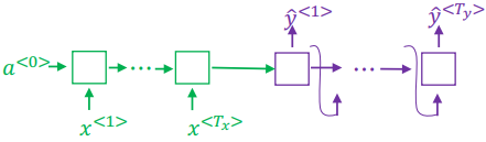
Notice that the encoder, in green, can use any type of RNN, GRU or even LSTM to learn some encoding of the entire input; that is, before generating any predictions we have seen the entire input and generated some encoding. From this learned encoding, the decoder part in purple, will generate each output $\hat{y}^{<t>}$, using the previous’ steps prediction for the next one until reaching the $T_y$ time step.
A very similar architecture works very well for image captioning, that is generating captions for an image. The idea is to have some trained CNN, something like AlexNet, and change the last layer; which in AlexNet is a softmax. We do this by replacing the softmax with some RNN, GRU or LSTM for generating the sequence of captions. Notice that this is very similar to the previous approach. The difference is that the CNN is acting as an encoder, while the sequence model is acting as the decoder.
Whatever approach we take, a question remains: how do we pick the most likely sequence? Can we cast this problem into a conditional probability one like we did before?
Picking the Most Likely Sentence
We can definitely think of machine translation as building a conditional language model. The difference being that we are not starting with a hidden state of $\vec{0}$, but instead we start the sequence generation from an encoding learned by the encoder network; just like the encoder-decoder image. In this case, our language model is the decoder.
Remember that in a language model, we try to model the probability of a sentence. We do this by using the conditional probabilities of each word as we move down in the sequence. So if the output sequence is I would like to have a balloon, and we are at the “balloon” step, we want our model to estimate the probability of seeing “balloon” given that it saw “I would like to have a” before. In machine translation we are doing the same except for a small change.
We would like to generate a sentence in the target language that maximizes the language model probability given that we saw the source language sentence (in its encoded form). In other words, we want to estimate:
$$ P(y^{<1>}, \dots, y^{<T_y>} \mid x^{<1>}, \dots, x^{<T_x>}) $$
Where $x^{<t>}$ is our source language sentence, and $y^{<t>}$ is our target language sentence.
How do we compare the likelihood of each of the sentences the model might consider? We might imagine that given the source language sentence Jane visite l’Afrique en septembre there might be many “likely” translations:
- Jane is visiting Africa in September.
- Jane is going to be visiting Africa in September.
- In September, Jane will visit Africa.
- Her African friend welcomed Jane in September.
Think of all these sentences as sampled from the $P(\underbrace{y^{<1>}, \dots, y^{<T_y>}}_{\text{English}} \mid \underbrace{x}_{\text{French}})$ distribution. Of course, all these probabilities should not be the same if your language model is modelling the translation task correctly. We want the best one:
$$ \argmax_{y^{<1>}, \dots, y^{<T_y>}} P(y^{<1>}, \dots, y^{<T_y>} \mid x) $$
Why not Greedy Search?
Finding the maximum should be easy, right? We just consider one at a time and then pick the highest one when we run out of elements. As you might know already, there’s an issue with this. Maximizing a linear function applied over a set of elements can be tricky; the knapsack problem is the quintessential problem that illustrates the issue. If we apply greedy search, and pick the most likely one at each step, we might not pick the set of words that together maximize the probability. That is, the problem is that the token that looks good to the decoder might turn out later to have been the wrong choice! 1
This approach is called greedy search, greedy of course because we greedily pick the largest value we find every time we look. Let’s think about the probabilities the model is modeling: we might see more common words sneaking into our translation when we don’t want it. For example a proper translation of the French sentence is Jane is visiting Africa in September. However, if we use greedy search, we might get results such as Jane is going to be visiting Africa in September, simply because going is more common than visiting. Notice that after picking going, all the other sentences picked after are also conditioned by this choice.
What else can we do? If we are not checking enough, let’s check them all. As you might imagine, considering the entire sequence at a time might result in an exponential explosion of checks. On one extreme, we have exhaustive search; which checks all possible permutations of the sequence with a time-complexity of $O(|V|^{T_y})$. If $|V| = 10000$ and $T_y = 10$ then exhaustive search will evaluate $10000^{10} = 10^{40}$ sequences. On the other extreme, we have greedy search; with a time-complexity of $O(|V|T_y)$; with the same numbers we would need $10000 \times 10 = 10^5$ sequence checks. 2 I hope you don’t need to be convinced that $10^5$ is a lot better than $10^{40}$.
It seems like neither approach would work. We’d like to use greedy search because it’s cheap, but it won’t work because there’s no guarantee of finding the optimal value. On the other hand, we’d like to use exhaustive search because it does guarantee finding the optimal value, but it’s computationally unfeasible. Wouldn’t it be nice to have something in between?
Beam Search
Beam search allows us to choose somewhere between greedy search and exhaustive search. It has a single hyperparameter called the beam size $B$, which controls how close we are to either greedy or exhaustive search. If we set $B=1$ then we are using greedy search, which means that if we set $B = k$ then we are considering $k$-best choices at each time. Let’s walk through the example shown in the course by Andrew.
Let’s start by trying to predict the first word in the output $P(y^{<1>} \mid x)$ and use $B = 3$. If we use greedy search, we would just pick the most likely word as $\hat{y}^{<1>}$ and set that for the next time step’s prediction. Since we are using $B = 3$, we will consider three different words, and not just any words, but the three most-likely tokens in the step. The $B$ most likely probabilities from the softmax at this step is called the search frontier, and the $B$ most likely tokens are called the hypotheses. Let’s say that for this step we get: [in, jane, september] as the $B$-most likely tokens. Let’s go into the next step.
Remember that we kept only 3 tokens in the past step since $B = 3$. For each of them we will calculate the conditional probability of the second token in the sequence:
- For
inwe calculate $P(y^{<2>} \mid x, \text{in})$ - For
janewe calculate $P(y^{<2>} \mid x, \text{jane})$ - For
septemberwe calculate $P(y^{<2>} \mid x, \text{september})$
Since our vocabulary size $|V| = 10000$ and $B = 3$ we will calculate $3 \times 10,000 = 30,000$ probabilities. It’s out of these $30,000$ probabilities that we will select the $B$ highest ones, that is, the three highest ones. Let’s say that the ones we pick are the following:
[in, september][jane, is][jane, visits]
Notice that we got rid of the third selection september in the first step as the first token in the output sequence. This is exactly what greedy search doesn’t allow us to do. Our decision to trade exploration for exploitation paid off! Now we just repeat the step again. Let’s say that we end up with:
[in, september, jane][jane, is, visiting][jane, visits, africa]
So on and so forth until one of the sentences predicts the end-of-sentence token, or we reach the maximum output sequence length.
Refinements
Since we are calculating conditional probabilities, and therefore all probabilities are $\in [0, 1]$, we don’t want our numbers to shrink so much and run into numerical underflow. The common trick to do this is to transform a multiplication into summation. Remember one of the properties of logarithms is that the log of a product is the sum of the logs: $\log_a xy = \log_ax + \log_ay$. Therefore, instead of calculating:
$$ \argmax_y \prod_{t=1}^{T_y} P(y^{<t>} \mid x, y^{<1>}, \dots, y^{<t - 1>}) $$
Where $\prod$ is the product symbol, much like $\sum$ is the summation symbol; we want to calculate:
$$ \argmax_y \sum_{t=1}^{T_y} \log P(y^{<t>} \mid x, y^{<1>}, \dots, y^{<t - 1>}) $$
This trick is found pretty much anywhere you are calculating conditional probabilities.
There’s another issue however, related to the length of the output sequence $y$. Since we are multiplying probabilities, or summing them in log space, longer sequences will have smaller probabilities assigned to them. This is simply because we are multiplying numbers between $[0, 1]$; $0.5^3 = 0.125$ while $0.5^2 = 0.25$. To ameliorate this, we will introduce a weighting term that normalizes the probabilities by the size of $T_y$
$$ \argmax_y \frac{1}{T_y^{\alpha}}\sum_{t=1}^{T_y} \log P(y^{<t>} \mid x, y^{<1>}, \dots, y^{<t - 1>}) $$
Setting $\alpha = 0.7$ to be somewhere in between $\alpha = 0$, no normalization, and $\alpha = 1$, full normalization.
Finally, regarding the beam size. As we mentioned, setting $B=1$ amounts to greedy search, which is fast but worse result. As we increase $B$, we get slower performance but better results. $B$ is a parameter that regulates the mixture of exploitation and exploration. Remember that to find exact maximums we need to use exhaustive search. Anything other than that has no guarantees. In beam search, we can adjust how much “guarantee” in finding an optimal solution by varying $B$.
Error Analysis
Since we introduced another source of error by using beam search, we need to be able to know whether errors are coming from the sequence model, or if they are arising from using beam search. That is, do we need to keep training/add more data, or do we need to use a larger beam size?
Let’s keep using the French example: Jane visite l’Afrique en septembre. Let’s say that the human-generated label in our dev set for this example is:
- $y^*$: Jane visits Africa in September.
And let’s say that our algorithm is predicting:
- $\hat{y}$: Jane visited Africa last September.
Obviously, our algorithm’s prediction is wrong! The whole meaning of the sentence is different. How can we zone-in into the root cause of the problem?
We can grab the RNN component of our model, that is the encoder and decoder, which computes $P(y \mid x)$, and compare two things:
- Run $y^*$ through the RNN, to estimate $P(y^* \mid x)$.
- Run $\hat{y}$ through the RNN, to estimate $P(\hat{y} \mid x)$
What are we really doing here? We are saying: Hey RNN! Do you think the bad translation is more likely than the good translation? If the RNN is predicting the bad translation to be more likely than the good translation, then it doesn’t matter what beam search is doing; the model still needs more training. On the other hand, if the model thinks that the good translation is more likely than the bad one, then the only way we are getting a bad translation at the end is due to beam search. In this case, increasing the beam width should help improve our model’s performance. In practice, we calculate the fraction of errors due to either the RNN or the beam search, and take action based on what is more efficient.
Attention
Through this whole week we have been using the encoder-decoder architecture, one RNN reads in the sentence and learns an encoding, while another RNN decodes the encoding. There is another approach, called the attention mechanism approach, which makes this work a lot better albeit for larger compute costs.
Developing Intuition
Let’s consider what happens in very long sequences, say a paragraph, when we try to apply machine translation with the encoder-decoder architecture. The encoder will memorize the entire thing, which is pretty long, and then pass it into the decoder. Think instead, how a human translator would tackle the problem of translating a whole paragraph. The translator might start with the first few sentences, translate them, and then move on. Even more so, the translator can read the entire paragraph before starting to translate, using the latter context of the paragraph to guide the beginning of the translation.
The encoder will try its best to encode as much useful information in the encoding, but as sentence length grows, this task gets harder and harder. In practice, the encoder-decoder architecture’s performance suffers as sentence length grows because of this. The attention approach is a remedy for this issue; the performance is not hurt as sentence length grows.
In the attention model, we no longer have an encoder-decoder architecture. Instead, we have a bidirectional RNN (choose your flavor) called the pre-attention RNN. Hooked to each of the outputs of the pre-attention bidirectional RNN, we will have a uni-directional RNN (choose your flavor) called the post-attention RNN. The role of the pre-attention RNN is to figure out how much attention to pay to each of the input words when predicting some word. Since the pre-attention RNN is bidirectional, we can pay attention to the entire input sequence when generating the first prediction.
We do this by learning some parameter $\alpha^{<t,t’>}$. Each parameter tells us, how much attention (a value $\in [0, 1]$) we should give French word $t’$ when generating the English word $t$. Let’s go into more detail.
Defining the Attention Model
Let’s start with the pre-attention bidirectional RNN, which in practice is usually implemented as a bidirectional LSTM network. Remember that in a bidirectional RNN, we have two hidden states $a^{<t>}$; one going forward $\overrightarrow{a}^{<t>}$, and one going backwards $\overleftarrow{a}^{<t>}$. To simplify the notation, we will define a single hidden state:
$$ a^{<t>} = (\overrightarrow{a}^{<t>}, \overleftarrow{a}^{<t>}) $$
Which is equal to both states concatenated together.
Let’s now focus on the post-attention RNN. This part will have a hidden state $s^{<t>}$, which is used to generate $\hat{y}^{<t>}$. What is the input of this post-attention RNN? It’s some context $c^{<t>}$ which is the output at step $t$ of the pre-attention bidirectional RNN. It’s this context which defines the attention mechanism.
The context will be the weighted sum of all $a^{<t>}$, the hidden state in the pre-attention layer, with their respective attention weights $\alpha^{<t, t’>}$. We want all attention weights for a particular token $t$ to sum up to one:
$$ \sum_{t’=1}^{T_x} \alpha^{<t,t’>} = 1 $$
We can then use these weights when calculating the context, we can control the mixture of each of the input tokens as it relates to this particular’s time step’s prediction:
$$ c^{<t>} = \sum_{t’=1}^{T_x} \alpha^{<t,t’>} a^{<t’>} $$
We should be convinced that when $\alpha^{<t,t’>} = 0$ it means that $t’$ is not that important when generating $t$, therefore the hidden state for $t’$ is not that important, and will be weighted down in the sum.
How do we calculate these attention weights $\alpha^{<t,t’>}$? Let’s be reminded that $\alpha^{<t,t’>}$ defines the amount of attention $y^{<t>}$ should pay to $a^{<t’>}$. We can define this attention as a softmax, to guarantee that the weights sum up to one as we mentioned earlier:
$$ \alpha^{<t,t’>} = \frac{\exp(e^{<t,t’>})}{\sum_{t’=1}^{T_x} \exp(e^{<t,t’>})} $$
But where do these new terms $e^{<t,t’>}$ come from? We will use a small neural network with only one hidden layer to learn these. The small network will take $s^{<t-1>}$ and $a^{<t’>}$ to produce $e^{<t,t’>}$. Let’s keep in mind that $s^{<t-1>}$ is the hidden state of the post-attention layer for the previous time step, while $a^{<t’>}$ is a hidden state in the pre-attention layer for the $t’$ time step. This means that this layer will learn to combine the hidden state of the previous token in the prediction, that is how relevant the previous prediction token is to the current one, with each of the input token hidden states, that is each of the tokens in the input.
It makes sense to define attention as: I have some memory of what I’ve translated so far, and attention is the thing that relates each of the words in the input, with the memory of what I’ve done so far. This means that $\alpha^{<t,t’>}$ and $e^{<t,t’>}$ will depend on $s^{<t-1>}$ and $a^{<t’>}$ when considering $t$.
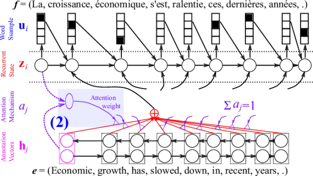
In the picture, the annotation vectors are the pre-attention layer, the attention mechanism represents the layer where we estimate $\alpha^{<t,t’>}$ and everything above the dotted line is the post-attention layer.
Next week’s post is here.