Sequence Models: Week 4 | Transformers

This is the fourth and last week of the fifth course of DeepLearning.AI’s Deep Learning Specialization offered on Coursera. The main topic for this week are transformers, a generalization of the attention model that has taken the deep learning world by storm since its inception in 2017.

This week’s topics are:

Transformer Network Intuition
Self-Attention
Multi-Head Attention
Transformer Network Architecture
More Information

Transformer Network Intuition Link to heading

We started with RNNs (known as part of the prehistoric era now), a simple model that reutilizes the same weights at each time steps; allowing to combine previous step’s hidden states with the current one. To solve some issues with vanilla RNNs, we introduced GRUs and LSTMs; both more flexible and more complex than simple RNNs. However, one of the things that they all share in common is that the input must be processed sequentially, i.e. one token at a time. This is a problem with large models, where we want to parallelize computation as much as possible. Amdahl’s Law gives us a theoretical speed up limit based on the fraction of parallelizable compute in a computer program. Unfortunately, since the entire model is sequential the speed-ups are miniscule. The transformer architecture allows us to process the entire input at once, and in parallel; allowing us to train much more complex models which in turn generate richer feature representations of our sequences.

The transformer architecture combines the attention model with a CNN architecture. The idea is to use the attention model’s ability to recognize relevance between pairs of tokens, with the computational efficiency of CNNs; which can be parallelized quite easily. Let’s dive into the two main components of the transformer architecture.

Self-Attention Link to heading

Self-attention is the same idea as attention when we used RNNs. However, since our model is not sequential anymore, we need to calculate the attention in one go. Let’s remember that attention is simply some value that describes how relevant a pair of tokens $<t,t'>$ are with respect to generating some output. In the RNN case, we learned some embedding $e^{<t,t'>}$ as a function of the previous step’s post-attention hidden state and each token $t'$ pre-attention hidden state. We no longer have previous hidden states since we are doing it all in one go. Let’s see how this implemented.

The first thing to take into account is that since our model is not sequential anymore, we have lost the temporal structure we got from using RNNs. This means that we will have to come up with a way to encode positions, which we will call the positional encodings. For now, just think that we have two things: our word embeddings from the input, and some positional encoding that encodes the position of each word in the sentence.

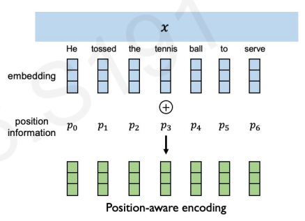
Notice that in the figure, we add the positional encoding to the word embeddings; therefore imbuing the embedding with positional information which was absent before.

Now we need to come up with a way to define attention. We can think of attention as a way for input nodes to communicate with each other. How can we imbue each node to talk with each other? We will define three things for each node in the input:

Key $k^{<t>}$: What do I have?
Query $q^{<t>}$: What am I looking for?
Value $v^{<t>}$: What do I publicly reveal/broadcast to others? ¹

Let’s define mathematically attention first, and then we will go over what each of these vectors represent:

$$ A^{<t>}(q^{<t>}, K, V) = \sum_{t'=1}^{T_x} \frac{\exp(q^{<t>}k^{<t'>})}{\sum_{j=1}^{T_x}\exp(q^{<t>}k^{<j>})} v^{<t'>} $$

Let’s use as an example, the input sentence Jane visite l’Afrique en septembre., and let’s focus on $x^{<3>} = \text{l’Afrique}$ and calculate $A^{<3>}$.

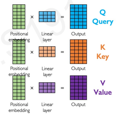
First, $q^{<3>}, k^{<3>}, v^{<3>}$ are generated with three weight matrices $W^Q, W^K, W^V$ which are learnable parameters:

$$ \begin{aligned} q^{<3>} &= W^Q x^{<3>} \\ k^{<3>} &= W^K x^{<3>} \\ v^{<3>} &= W^V x^{<3>} \end{aligned} $$

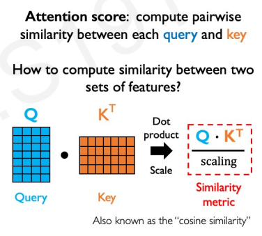
To compute $A^{<3>}$ we will allow $x^{<3>}$ to communicate to all other tokens what it’s looking for: $q^{<3>}$. Each of the tokens will respond with $k^{<t'>}$, answering what they have. This is the key part: if the dot product between $q^{<3>}$ and $k^{<t'>}$ is high, it means that $k^{<t'>}$ has what $q^{<3>}$ is looking for; we are simply looking for a similarity between the query and key vectors. We will allow each token to communicate with all others, and then normalize their contributions with a softmax. We also use $v^{<t'>}$ to weight the contribution, allowing token $t'$ to not just say that it has what someone else is looking for, but what it is, regardless of what someone else is looking for. Finally, we sum all of these up into $A^{<3>}$. Let’s revisit these steps in more detail again.

Remember that we are doing all of this in one go, therefore we need to do this in a vectorized way using matrix multiplication. Let’s redefine attention with matrices:

$$ \text{Attention}(Q, K, V) = \text{softmax} \left( \frac{QK^T}{\sqrt{d_K}}V \right) $$

We get each of these matrices by multiplying the positional embeddings with each of the $W^Q, W^K, W^V$ matrices:

Let’s break down the matrix version of the attention formula. Let’s focus on this term:

$$ \frac{QK^T}{\sqrt{d_K}} $$

This term is calculating the pair-wise similarity between queries and keys for all the inputs:

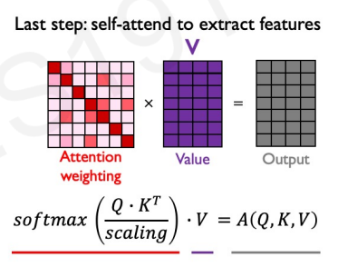
This means that we will have a matrix with the dimensions of our maximum input size, where each row and column corresponds to a position of the input. Along the diagonal, we will have the similarity between each token and itself. We would like to normalize the values to sum up to one (across some specific dimension!); we can use our trusty softmax to do that. We therefore get:

$$ \text{attention weighting} = \text{softmax} \left( \frac{QK^T}{\sqrt{d_K}} \right) $$

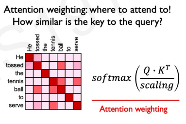
This matrix encodes which token is relevant for every token in the output. We know to which token to pay attention to, but what about that token do we pay attention to? This is what $V$ encodes. Multiplying the previous with $V$ allows us to extract features with high attention. We finally get to:

$$ \text{Attention}(Q, K, V) = \text{softmax} \left( \frac{QK^T}{\sqrt{d_K}}V \right) $$

If we do this for every token in our output and get $A^{<t>} \forall t \in T_x$ we will get an attention embedding for all the inputs. This constitutes a single head. It turns out that we will use a head similar to how we use a filter in the context of CNNs. This is the part that we can run in parallel, on top of the vectorization of the $A^{<t>}$ calculation. By using different heads, we allow the model to focus on different features when generating the queries, keys and values. That is we can learn to pay attention to different things, as many things as we have heads. This means that if we have $5$ heads, we will have $W_1^Q, W_1^K, W_1^V, \dots, W_5^Q, W_5^K, W_5^V$. This is called multi-head attention.

Multi-Head Attention Link to heading

Similar to how we can stack filters in a CNN to learn different features, we will stack multiple heads to learn different attention representations for each token pair. We know that attention a single-head attention is defined as:

$$ \text{Attention}(Q, K, V) = \text{softmax} \left( \frac{QK^T}{\sqrt{d_K}}V \right) $$

We will index each head with the subscript $i$ so that:

$$ \text{head}_i = \text{Attention}(W_i^Q, W_i^K, W_i^V) $$

This allows us to define multi-head attention as:

$$ \text{MultiHead}(Q, K, V) = \text{concat}(\text{head}_1, \text{head}_2, \dots, \text{head}_h)W_o $$

Notice that $W_o$ is another matrix with learnable parameters, which allows us to dial up or down the signal coming from the multi-head component.

We said that the transformer architecture allows for parallelization before, and this is exactly the part that runs in parallel. That is, every head runs the communication (attention) scheme in parallel.

Transformer Network Architecture Link to heading

Alright, let’s do a quick recap:

We have dealt with the loss of temporal structure by using positional encodings.
We have defined a way which allows nodes to communicate with each other, and learn to which of their friends to pay attention to.
We have done this $h$ times, the number of heads, to allow the nodes to ask different combinations of questions and answers: What do you mean? Where are you? Etc.

The output of this is some encoding of the input that has all this information clumped together into a super rich embedding of the inputs. This is what we call the encoder part:

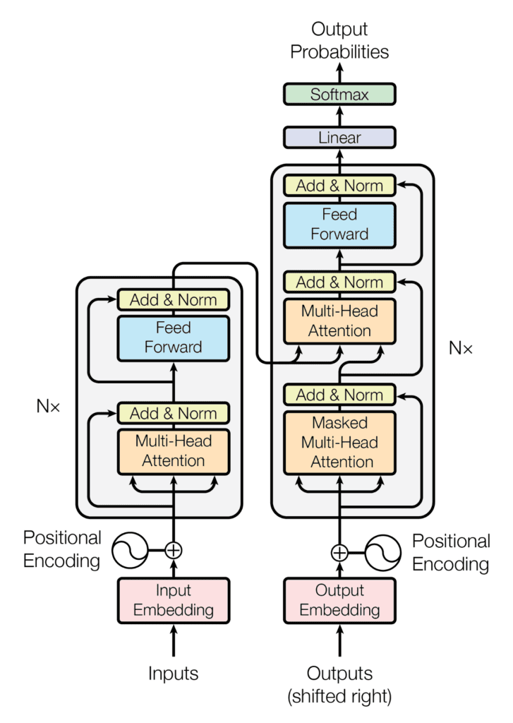
The three arrows in the encoder part (left) that go into the Multi-Head Attention component are the three query, keys and values matrices $Q, K, V$ for each of the heads. Remember, we learn $Q, K, V$ via optimization; and we have as many of these representations as we have heads. An additional step shown in the figure is that we add a skip connection with normalization; similar to how we implemented skip-connections in U-Nets.

What about the decoder? The decoder will take the inputs, but shifted to the right for each context length, and learn new $Q, K, V$ representations from the training labels. In machine translation, these are $Q, K, V$ in English instead of French. It will then be able to get its own questions $Q$ in English, and allow it to reach out into the encoder for finding keys and values. This is sometimes called the cross-attention module. After this, we run the embeddings through a feed-forward layer to select the most important features and generate the softmax probabilities for the next token in the prediction.

Transformer Network Intuition Link to heading

Self-Attention Link to heading

Multi-Head Attention Link to heading

Transformer Network Architecture Link to heading

More Information Link to heading