This is the first week of the fifth course of DeepLearning.AI’s Deep Learning Specialization offered on Coursera. This week we go over some motivation for sequence models. These are models that are designed to work with sequential data, otherwise known as time-series. Let’s get started.
This week’s topics are:
- Why Sequence Models?
- Notation
- Recurrent Neural Network
- Gated Recurrent Unit
- Long Short-Term Memory
- Bidirectional RNN
Why Sequence Models?
Time-series get to be their own thing, just like in regression analysis. This time, since we are focusing on prediction instead of inference, we are less concerned about the statistical properties of the parameters we estimate, but we’d like our models to do very well in their prediction tasks. But how can we exploit temporal information, without using classical methods such as AR methods? The current bag of tricks we have developed so far will only take us some distance. Here are a couple of hiccups:
- Vanilla neural networks require all training samples $X$ to be of the same length. What happens when we want to use text as input and each sample can have different length? Sure we can pad, but I hope you’re convinced that’s not a great idea from the get go.
- Vanilla neural networks treat every feature $x^{(i)}_i$ as independent. The whole point of time-series is that they have two components: time-invariant and time-variant components. We definitely want to exploit the temporal structure of our data, which the vanilla models won’t allow us to.
- Vanilla neural networks with dense layers explode very quickly in their size. We need some approach, similar to that of CNNs, where parameters are shared to have a feasible approach in terms of computation.
Before we get to the thick of it, let’s define the notation used in the course and disambiguate some terminology as well.
Notation
Our input will be, as usual, some vector of features. We denote each time step with $t$, so that $x^{<t>}$ is the $t_{th}$ element in our input vector. We also denote the $i_{th}$ training example as $x^{(i)}$, so that $x^{(i)<t>}$ denotes the $i_{th}$ training example’s $t_{th}$ time step. Similarly, we will also denote the size of our input with the variable $T_x$. All of this applies also to our labels $y$. Sometimes $T_x = T_y$, and sometimes it’s not. We will discuss these variations under the different types of RNNs.
Representing Words
Since a lot of sequence models deal with words, we need a handy way of representing words and even sentences. We need to start by defining a vocabulary. A vocabulary is simply the set of all words in our corpus. A corpus is natural-language processing equivalent to a dataset. If we are training a model on data scraped from news sites, then all the news articles we scraped will make our corpus.
Since we have a set of all words in our corpus, more precisely tokens in our corpus, we can assign each word a number. This number is the position of the word in our vocabulary. For example, the word aaron might be in position $2$, while the word zulu might be in position $10,000$. This is assuming that our vocabulary is sorted and that it’s size, or cardinality is $10,000$.
We can now transform every word in a sentence into a one-hot vector. This simply means creating a vector of size equal to our vocabulary, that is $10,000$ and fill it with zeros. Next, we get the index of a word from our vocabulary, and set that index’s element in our vector to $1$. So that every word is represented by a $10,000$ dimensional vector where all the entries are $0$ except for the position that maps to a word in our vocabulary. More precisely, we can represent each element in our input $x^{<t>}$ as a one-hot vector. Thus, a sentence can be represented by a matrix, where we concatenate each word. If we have a sentence with $20$ words, then our representation will be of dimensions $(10000, 20)$.
Since we can also represent some output sequence $y$ in the same fashion, we will use supervised learning to learn a mapping that goes from $x \to y$.
As we mentioned before, there are two main issues with using a standard neural network approach with sequence data.
- Input and outputs can be of different lengths between them and also across training examples.
- Does not share features across different positions of the sequence. Every element is processed independently of another, which is a pretty bad approach since we are dealing with data that is intrinsically linked in time.
We can solve both these issues using a surprisingly simple model, a recurrent neural network (RNN).
Recurrent Neural Network
RNNs is an architectural approach that allows us to express our desire to share parameters, and also to generalize input and output lengths. Let’s define that.
At each step an RNN will take some input $x^{<t>}$, combine it with the activations (hidden state) from the previous time step $a^{<t-1>}$, and generate $a^{<t>}$. It will use $a^{<t>}$ to generate some output $\hat{y}^{<t>}$ and also pass $a^{<t>}$ to the next layer $l^{<t+1>}$ to repeat the process again. This means that at each time step we are putting in an input, combining it with the activations from the previous layer and generating an output; so on and so forth until we reach the end of the time steps. Andrew mentions that a lot of the diagrams from RNNs, and later GRUs and LSTM networks, are hard to understand. In that spirit I will focus more on the equations because they are clearer to me.
A key thing to take note of is that we are sharing parameters across all time steps. There are three important parameter matrices: $W_{ax}$, $W_{aa}$ and $W_{ay}$. In the notation of the course, the subscripts $W_{ax}$ denote that this particular $W$ is being used to generate $a$, and it’s using $x$. This means that $W_{ax}$ is used to combine the inputs $x^{<t>}$ and generate $a^{<t>}$. Similarly, $W_{aa}$ is also used to generate $a^{<t>}$, but it uses $a^{<t-1>}$, the activations from the previous time step. This will become clearer once we go over the equations. However, just keep in mind that we have three knobs (parameter matrices):
- $W_{ax}$: regulates how each $x^{<t>}$ affects the activations $a^{<t>}$.
- $W_{aa}$: regulates how the activations from the previous layer $a^{<t-1>}$ affect our current activations $a^{<t>}$.
- $W_{ay}$: regulates how the activations $a^{<t>}$ are combined into the current output $\hat{y}^{<t>}$.
Notice that these three matrices are reused at every time step. This means that our parameters will not grow or shrink with respect to the length of our output or input sequences.
Also notice the main point of RNNs: as long as $t > 1$ then the output $y^{<k>}$ will be computed using all time steps $t_1, \dots, t_k$. That is, the future is affected by the past (but not the other way around). If you’re interested doing away with the arrow of time, you can use bidirectional RNNs, but that comes later.
Forward Propagation
Let’s finally define the equations that govern the forward pass in an RNN and hopefully do away with ambiguities in the writing.
We said that at every time step, an RNN combines the hidden state from the previous time step with the current inputs to generate an output. How do we get started? That is, what do at $t = 0$? We initialize the hidden state, $a^{<t>}$ to be the zero vector, therefore $a^{<0>} = \vec{0}$. Thus, we can define the general form of the forward propagation equation:
$$ \begin{aligned} a^{<t>} &= g_a (W_{aa} a^{<t - 1>} + W_{ax} x^{<t>} + b_a) \\ \hat{y}^{<t>} &= g_y (W_{ya} a^{<t>} + b_y) \end{aligned} $$
Notice the activation functions $g_a, g_y$ might be different. In practice, we use the $\tanh$ for $g_a$ and the sigmoid for $g_y$ in the case of classification.
These two operations are all that’s going in an RNN, repeated for every time step of the output. As mentioned before, keep in mind that $T_x = T_y$ for now.
Another thing done in the course is to simplify the notation of the equation above, by concatenating $W_{aa}$ and $W_{ax}$ together. For example, if $W_{aa}$’s dimensions are $(100, 100)$ and $W_{ax}$’s dimensions are $(100, 10000)$, then we can concatenate these into $W_a$. So that:
$$ \underset{(100, 10100)}{W_a} = \left[\underset{(100, 100)}{W_{aa}} | \underset{(100, 10000)}{W_{ax}}\right] $$
Similarly, we can stack $a^{<t-1>}$ and $x^{<t>}$ to match the dimensions of $W_a$. So that:
$$ \underset{(10100, 1)}{\left[ a^{<t-1>}, x^{<t>}\right]} = \begin{bmatrix} \underset{(100, 1)}{a^{<t-1>}} \\ \hline \\ \underset{(10000, 1)}{x^{<t>}} \end{bmatrix} $$
This way we can simplify the activation function to:
$$ a^{<t>} = g_a (W_a \left[ a^{<t-1>}, x^{<t>}\right] + b_a) $$
Which is what we’ll use through the rest of the week. Notice that this is just a notational trick and also to keep all hidden state parameters together into a single matrix. We are not adding or removing any parameters by doing this notational refinement.
Different Types of RNNs
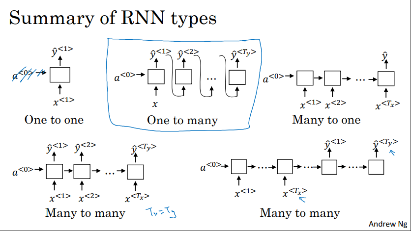
It turns out that setting $T_x = T_y$ is pretty restrictive. We can have different types of RNNs that have different sizes for their input and output. We have the following:
- Many-to-one approach: In sentiment classification we take a sequence and want a single output. We do this by editing the usual RNN approach. Instead of having an output at every time step, $\hat{y}^{<t>}$, we only have one at the end. A key thing is that we still keep the hidden state going through each time step like a regular RNN.
- One-to-many approach: In a case like music generation, we might input a single thing, such as a chord, and would like to generate a sequence based on this. This is the mirror opposite of the many-to-one approach. We still have one output at each time step $\hat{y}^{<t>}$, but we only have one input at the first time step.
- Many-to-many approach: In this approach, we have two cases:
- $T_x = T_y$: This is the usual approach. Each RNN unit takes in an input and produces an output.
- $T_x \neq T_y$: This approach is usually used in machine translation. The idea is that you first have an encoder, and then a decoder. The encoder takes the inputs and learns an encoding of the inputs, still passing the hidden-state forward in time. While the decoder generates the outputs.
Here is an image from the course:
Language Model and Sequence Generation
Language modeling is a probabilistic model of natural language that can generate probabilities of a series of words, based on text corpora in one or multiple languages it was trained on. 1 This means that for a given sentence, our a language model should be able to estimate the probability of that sentence occurring in our corpus. Notice that we can estimate probabilities for sentences that were not seen during training.
If we have a sentence such as “Cats average 15 hours of sleep a day.”, then we can model each token as a one-hot vector. Our tokens will be [cats, average, 15, hours, of, sleep, a, day, <eos>], where <eos> is a special token that denotes the end of sentence. This is useful, because we want our model to be able to learn when it’s likely for a sentence to end. We can see how the RNN approach can be used almost directly to estimate the probabilities of this sentence.
Imagine that we train an RNN with the same settings as before, and that we trained it on a large English corpus. Also keep in mind that we want to set $x^{<t>} = y^{<t-1>}$. What happens in the first time step? We just set $x^{<1>}$ to be $\vec{0}$. If we run this through the first RNN unit, we will get a softmax output over the entire vocabulary. That is, $P(x) \forall x \in V$ where $V$ is our vocabulary. We can grab the most likely word, or sample the vocabulary used the softmax probabilities, and generate $x^{<2>}$ from what we just estimated from $y^{<1>}$, so on and so forth.
The important idea behind this is that, using an RNN like this amounts to calculating the conditional probabilities for each of the words in the sentence. For example, $y^{<1>} = P(y^{<1>})$, $y^{<2>} = P(y^{<2>} | y^{<1>})$ and so on. When training the neural network, we use the following loss function:
$$ J\left(\hat{y}^{<t>}, y^{<t>}\right) = - \sum_{i=1}^m y_i^{<t>} \log \hat{y}_i^{<t>} $$
Which is the cross-entropy loss we are already familiar with. Therefore, our cost function is just the sum over all time steps:
$$ \mathcal{L} = \sum_{t=1}^{T_y} J^{<t>}\left(\hat{y}^{<t>}, y^{<t>}\right) $$
This means that the model learns how to assign probabilities to sentences using conditional probability. For example the second output $\hat{y}^{<2>} = P(y^{<1>}) P(y^{<2>} | y^{<1>})$, the third output gives us $\hat{y}^{<3>} = P(y^{<3>} | y^{<1>}, y^{<2>})$. Since we are computing the loss with the sum of cross entropy, we are multiplying all these probabilities (summing in log space) to get the conditional probability of all these words together, given the ones that came before. This is why we can use an RNN as a language model. Even more so, we can generate novel sequences by using the output from one time step into the next step. Notice that we didn’t do this just now, we passed the target label from the previous time step to the next input time step.
Vanishing Gradients with RNNs
It turns out that vanilla RNNs suffer greatly from vanishing gradient problems. This might not be surprising since each RNN unit is like a layer, and therefore part of the chain rule when we do back propagation. In English, this means that the network is not very good at capturing long-term dependencies in a sequence. For example, in the sentence “The cat, which already ate an apple, was full”, when compared to “The cats, which already ate an apple, were full” has a long-term dependency. If it’s not clear, the dependency is between the pair $(\text{cat}, \text{was})$, and $(\text{cats}, \text{were})$. We still have not gotten to bidirectional RNNs, so the network is only scanning from left to right. This means that our optimization algorithm will have a harder and harder time updating the weights of the elements in the sequence that are further from the output towards the beginning of the sequence. This is what we mean by vanishing gradients in this problem.
In practice, a vanilla RNN implementation has high local dependencies. This means that some output at time step $t$ will be greatly influenced by the activations from the neighboring time steps before, but not much, if at all, by the ones further behind. This is of course, a problem. We want our language model to realize that seeing either cat or cats should affect the probabilities in the rest of the prediction, and also to memorize this fact as it keeps going down the sequence.
We can also have exploding gradients in some cases, which we can ameliorate with gradient clipping. That is, we restrict the gradient values to be within some arbitrary range chosen by us.
Gated Recurrent Unit
The Gated Recurrent Unit (GRU) is an improvement over vanilla RNNs that deals with the problem we just discussed, that of vanishing gradients, and therefore the lack of long-term dependency recognition. Before we define the GRU approach, let’s go back to how the regular RNN calculated the activations for some time step $t$:
$$ a^{<t>} = \tanh (W_a \left[ a^{<t-1>}, x^{<t>}\right] + b_a) $$
Where we simply replaced $g_a$ to use the $\tanh$ activation function. Let’s talk about what $W_a$ is doing. The part that’s multiplied with $a^{<t-1>}$ are the parameters that regulate how much the hidden state influences the activation, while the part that’s multiplied with $x^{<t>}$ are the parameters that regulate how much each new input sequence influences the activation. That is, in a vanilla RNN each activation is a combination of the hidden state from the previous time step, and the current time step’s input.
What the GRU does, is that it allows us to parametrize the mixture between hidden states and the activation; this is on top of $W_a$. The mechanism that performs the mixture is the gate, which is where the name comes from. The gate can be full, closed or anything in between, think sigmoid. When it’s open, the mixture from the past is heavy, when it’s closed, the mixture from the past is light. Let’s clarify this with math.
Let’s say that $c$ is a memory cell, and that in this case $c^{<t>} = a^{<t>}$. We will also define a candidate memory cell $\tilde{c}^{<t>}$:
$$ \tilde{c}^{<t>} = \tanh (W_c \left[ c^{<t-1>}, x^{<t>}\right] + b_c) $$
So far it’s the same as before but with other variable names. Now, we introduce the update gate:
$$ \Gamma_u = \sigma (W_u \left[ c^{<t-1>}, x^{<t>}\right] + b_u) $$
Let’s keep in mind some properties of $\Gamma_u$:
- $W_u$ are the parameters that we learn by optimization.
- The sigmoid guarantees values between $0$ and $1$.
- The gate has the same dimensions as the hidden state $c^{<t-1>}$. This means that element-wise multiplication can be used.
- This is similar to applying a mask, but instead of a binary one, a continuous one because of the sigmoid activation.
- If the value of the gate at some position is close to $0$, then the product is close to $0$ which dampens the effect of the previous hidden state into the next time stamp.
- On the other hand, we can heighten the hidden state’s effect into the next time stamp.
We’d like to add this gate to the $c^{<t>}$ equation. We can do this by:
$$ c^{<t>} = \Gamma_u \tilde{c}^{<t>} + (1 - \Gamma_u) c^{<t-1>} $$
So that at every activation, we are generating the candidate, and applying the gate over it; thus generating the final activations for the current unit. This means that a GRU not only learns how to mix the past and the present, but also how some tokens or inputs can be “context switches”; and also how some are not context switches. This means that the model can learn longer-term structural information over a sequence. If there’s a token that conditions the rest of the sequence, then the model can learn to update or open the gate. Otherwise, it can learn to keep the gate shut, thus enlarging or diminishing the effect from the past.
A key thing to note is the element-wise application of the gate. This means that the gate operates at the dimension level, instead of the input level. This means that the network can selectively update some dimensions more aggressively than other dimensions.
It turns out that the actual GRU unit has two gates, instead of one; but it’s literally the same principle. The full GRU equations are:
$$ \begin{aligned} \Gamma_r &= \sigma (W_r \left[ c^{<t-1>}, x^{<t>}\right] + b_r) \\ \tilde{c}^{<t>} &= \tanh (W_c \left[\Gamma_r c^{<t-1>}, x^{<t>}\right] + b_c) \\ \Gamma_u &= \sigma (W_u \left[ c^{<t-1>}, x^{<t>}\right] + b_u) \\ c^{<t>} &= \Gamma_u \tilde{c}^{<t>} + (1 - \Gamma_u) c^{<t-1>} \end{aligned} $$
The gate $\Gamma_r$ is the “relevance” gate. It’s a parameter that regulates how relevant the previous memory cell $c^{<t-1>}$ is in the next time step. While $\Gamma_u$ is the “update” gate. A parameter that regulates how relevant our candidate memory cell is relative to the previous memory cell.
Note that in the literature $c$ and $\tilde{c}$ are usually referred as $h$ and $\tilde{h}$. Similarly, $\Gamma_u$ and $\Gamma_r$ are referred to as $u$ and $r$ respectively.
Long Short-Term Memory
Long Short-Term Memory (LSTM) units are the extension of the GRU idea, even though LSTMs were published earlier. Let’s start by reviewing the equations for GRUs since the LSTM is a small extension of them.
For the GRU we have:
- Candidate for replacing the current memory cell: $\tilde{c}^{<t>} = \tanh (W_c \left[\Gamma_r c^{<t-1>}, x^{<t>}\right] + b_c)$
- The relevance gate: $\Gamma_r = \sigma (W_r \left[ c^{<t-1>}, x^{<t>}\right] + b_r)$
- The update gate: $\Gamma_u = \sigma (W_u \left[ c^{<t-1>}, x^{<t>}\right] + b_u)$
- The current memory cell: $c^{<t>} = \Gamma_u \tilde{c}^{<t>} + (1 - \Gamma_u) c^{<t-1>}$
- Which is a mixture of the current memory cell and the candidate memory cell mixed by the update gate.
- $a^{<t>} = c^{<t>}$
- This is something that will change in the LSTM.
In the LSTM we get rid of $\Gamma_r$, but we introduce two other gates: $\Gamma_f$ and $\Gamma_o$, the forget gate and output gate respectively.
For the LSTM we have:
$$ \tilde{c}^{<t>} = \tanh (W_c \left[a^{<t-1>}, x^{<t>}\right] + b_c) $$
Notice how we are back to using $a^{<t>}$ instead of $c^{<t>}$, and also that we dropped $\Gamma_r$ which we will redefine in a second.
The update gate remains the same, albeit with the input change:
$$ \Gamma_u = \sigma \left(W_u[a^{<t-1>}, x^{<t>}] + b_u\right) $$
We dropped $\Gamma_r$ but only to redefine it more explicitly as $\Gamma_f$, the forget gate:
$$ \Gamma_f = \sigma \left(W_f[a^{<t-1>}, x^{<t>}] + b_f\right) $$
We will add yet another gate, same as the others, $\Gamma_o$ the output gate:
$$ \Gamma_o = \sigma \left(W_o[a^{<t-1>}, x^{<t>}] + b_o\right) $$
The current memory cell will now use both $\Gamma_u$ and $\Gamma_f$ instead of $\Gamma_u$ and $(1 - \Gamma_u)$:
$$ c^{<t>} = \Gamma_u \tilde{c}^{<t>} + \Gamma_f c^{<t-1>} $$
Finally, we use the output gate $\Gamma_o$ to generate the final activations:
$$ a^{<t>} = \Gamma_o c^{<t>} $$
What does the LSTM get us for the extra size? It gets us more complexity and adaptability. By using more gates, and by keeping the hidden state and the output separate, we are subdividing the tasks more finely than in the GRU; therefore being able to achieve greater specialization.
Bidirectional RNN
Bidirectional RNNs (BRRNs) are simply running time forward and backward before doing a prediction. That is, before generating the first output, we’ve seen the entire sequence. By keeping two hidden states, one for forward in time, and the other for backwards in time, and then combining both these states with the input, we can use information from the future to make a prediction now. Computationally it’s almost two times as expensive as a single RNN.
In practice many people use bidirectional GRUs or LSTMs to also allow the model to parametrize the mixture over longer periods of time.
Next week’s post is here.