Here we kick off the second week of the first course in the specialization. This week is very technical, and many of the details shown in the course will be lost in the summarization. Also, a lot of the content is based on you doing programming assignments. There is simply no substitute for getting your hands dirty.
This week’s topics are:
- Binary Classification
- Logistic Regression
- Logistic Function
- Gradient Descent
- Computation Graph
- Python and Vectorization
- Broadcasting
Binary Classification
Binary classification is a supervised learning approach where you train what’s called a classifier. The binary classifier is a model that learns how to discriminate between two classes from the features, think about cats and dogs. A key concept is that of linearly separability:
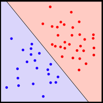
The existence of a line separating the two types of points means that the data is linearly separable
This is a property of your training data, some datasets are linearly separable and others are not. You can a have a linear binary classifier that works perfectly if the data is linearly separable, and this is what a perceptron can do, the building blocks of neural nets. However, if you imagine a dataset where there is no line that separates the classes then you need a non-linear classifier, which is extremely common when you work with data in the wild. There are two main ways of adding non-linearities to a linear classifier: use a kernel classifier, or you can add a single hidden layer to a perceptron, making it into a neural network. One of the best demonstrations of this principle is in creating a classifier that works on the XOR problem. It turns out that the latter is much more versatile.
Logistic Regression
A basic perceptron can be a linear classifier, but by itself it cannot tell you how uncertain it is about a particular prediction. If dogs are labeled as $0$ and cats as $1$, then you don’t want ones and zeros, but actually a probability that a training sample is a cat (or a dog depending on the positive class). We can define what we want our prediction to be:
$$ \begin{equation} \hat{y} = P(y = 1 \mid x) \end{equation} $$
Where $\hat{y}$ is the probability that a picture of a dog or cat $x$ is actually a cat, $y=1$, given a particular picture $x$. We will never know the exact probability $y$ (a parameter), so we denote our estimate with a hat $\hat{y}$ (a statistic). Logistic regression achieves this by composing two things:
- Linear regression
- Logistic function
Linear regression is a way of fitting a line (or plane, or something as you go up higher dimensions) to some data. The line (or plane, etc.) will be a line that minimizes some measurement of error, usually the euclidean distance between a point, and it’s prediction. You can describe a line with two parameters, it’s intercept $b$, and it’s slope $w$. Linear regression finds $\hat{b}$ and $\hat{w}$ such that they minimize some loss or error. You can describe linear regression as a linear combination of your features and the parameters:
$$ \begin{equation} y_i = \mathbf{x}_i^Tw + b \end{equation} $$
It turns out that under some assumptions, linear regression has a closed form solution, which simply means that you can take out a pen and do algebra and solve for a set of linear equations using least squares. The next step will undo our ability to have a closed-form solution. If you’re into economics you might now this and much more by heart, but to the extent of this course, it’s enough to know that we have a way of fitting a line (linear classifier) to our data, and that it has a closed-form solution.
Logistic Function
We now have a way of fitting a line to our data. However, that line’s domain, it’s range of values, ranges over all the real numbers $\mathbb{R}$. Our linear regression could output any number, but we want probabilities. It turns out that there is a nice way to map the real numbers $\mathbb{R}$, or the interval $[-\infty, \infty]$ into the interval $(0, 1)$. You can do this with a type of sigmoid function, called the standard logistic function:
$$ \begin{equation} \sigma(x) = f(x) = \frac{1}{1+e^{-x}} \end{equation} $$
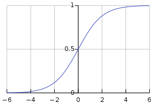
If $x$ is large, then $\sigma(x) \approx 1$, if $x$ is small, then $\sigma(x) \approx 0$, and everything in between in a continuous fashion. This is how we get our probabilities. Remember that any number $x^0 = 1$ so when $x = 0$ then $\sigma(0) = 0.5$
Logistic regression combines the two in a very literal way:
$$ \begin{equation} P(y = 1 \mid x) = \hat{y} = \sigma(\mathbf{x}_i^Tw + b) \end{equation} $$
We literally just pass our linear regression estimate through a sigmoid function. It turns out that we no longer have access to a nice closed-form solution. This means that we will need to find the parameters $w, b$ via numerical optimization. Now, how do we know this amounts to estimating the probabilities? There is a lot of work done on this, under the name of maximum-likelihood estimation (MLE). For now assume that what you get out are estimates of the probabilities.
Let’s pack our model’s parameters $w, b$ into a single vector $\theta$, so that $\theta_0 = b, \theta_1 = w_0$, etc. Now we can have many parameters, one for each feature in our input, so that feature $i$ maps to $\theta_{i+1}$ since $b$ is an additive constant. Now our logistic regression looks like this:
$$ \begin{equation} P(y = 1 \mid x) = \hat{y} = \sigma(\theta^TX) \end{equation} $$
Where $X$ is a matrix representing our data, each sample in a row, and each feature as a column.
Gradient Descent
To recap, we have combined a linear regression with a sigmoid function with the purpose of getting an estimate of the probability that an image is a cat. We know that there is no closed-solution to the equation, and that we need to find the parameters via optimization. Gradient descent does this for us. There is a ton of amazing gradient descent content online, so I will skip a lot of details.
In a nutshell, gradient descent is what fuels the “learning”. This is how the model is able to estimate the parameters from the training data, in our case $\hat{\theta}$. It starts with $\hat{\theta}$ chosen at random (more on this later), and then it runs a training sample through our logistic regression function. Then it compares the predicted value with the actual value, $(\hat{y_i}, y_i)$ using a loss function, $\mathcal{L}(\hat{y_i}, y_i)$. The loss function tells us how bad a single prediction is. We get to be very creative with our loss functions, although many loss functions are well established for certain applications. On top of this, we have a cost function $\mathcal{J}(\theta)$, which computes the loss for our entire training set using a specific set of parameters.
Finally, gradient descent does its magic. Gradient descent will differentiate $J(\theta) = \sum_{i = 1}^m\frac{1}{m}\mathcal{L}(\hat{y_i}, y_i)$, our cost function averaged across our training set, with respect to $\hat{\theta}$, our current estimate of $\theta$ (some random numbers currently). Remember that differentiation describes the rate of change between some function parameter and its output. In this case, we want to know how perturbing or changing $\hat{\theta}$, our parameters, changes $J(\theta)$, how bad our prediction is. If $\theta$ is a knob in our machine, we want to know which way to turn the knob to make our predictions better. This is what gradient descent does for us. It figures out in which direction our predictions become better with respect to $\theta$, and then it takes a step (moves the knob) in the direction that minimizes our loss (how we want the machine to work). Then it repeats this steps many times, called iterations, until we converge to a minimum. The basic version of gradient descent uses the entire dataset for each iteration, and it calculates a cost function $J(\theta)$ which is the loss of our predictions averaged across the entire dataset.
The name gradient descent comes from the fact that a gradient is simply the vector version of a derivative. Whereas the derivative is usually a scalar (single number), the gradient $\nabla f(\mathbf{x})$ is a vector describing how $f$ changes with respect to every element $x_i$ of $\mathbf{x}$. Since at every iteration we are “taking a step” towards a lower (better) cost, it’s a descent.
All of this is done via basic calculus, using derivative rules. In the case of logistic regression, this is relatively easy to do. But in the case of neural networks, where we stack these logistic regression on top of each other, the calculus gets very messy.
Computation Graph
Since the calculus gets very messy, we might as well get a machine to do it for us. We describe this process to a machine via a computational graph; this is simply an ordering of the mathematical operations in our neural network. This particular ordering can be differentiated step by step using the basic rules of differentiation. This is nice because as our neural networks grow deeper, the computational graph also grows bigger and so more computation is required. The process described just now is called automatic differentiation, and it’s the core of modern deep learning software like PyTorch or TensorFlow.
With a computation graph and a way to calculate the derivatives, we can unleash gradient descent on our data. The basic steps are:
- Forward propagation: Calculate the output of our model with the current $\hat{\theta}$
- Backward propagation: Calculate the gradient of our cost function $J(\theta)$ with respect to our current estimates $\hat{\theta}$ and then update $\hat{\theta}$ (via calculus) towards the minimum cost by some amount (the learning rate).
- Rinse and repeat
Python and Vectorization
This section shows you how to actually code these things from scratch in a relatively efficient manner. I say relatively, because in practice (or production to borrow a fancy term), you will almost never code these things up from scratch. Don’t reinvent the wheel (unless you think the wheel is obsolete). You will most likely implement a neural network using a mature software package such as PyTorch or Tensorflow. There are still key ideas that are important to discuss.
Vectorization or array programming, simply means applying a single operation to many pieces of data, it’s a $1:M$ operation where $M$ is the size of an array. For example, this is a $1 : 1$ operation:
>>> "w".upper()
"W"
A $1:M$ operation:
>>> "".join(map(str.upper, "Hello, World!"))
"HELLO, WORLD!"
In Python, strings are sequences of characters, therefore they are iterable. What the code above does is it applies the str.upper method to all the elements of a string.
This is technically vectorization, but in general, the term vectorization usually refers to math and linear algebra operations. If we have two vectors $x, y$ both of size $3$, and we want to calculate the dot product between the two, we would have to write a loop:
x = [1, 2, 3]
y = [1, 2, 3]
total = 0
for left, right in zip(x, y):
    total += left * right
print(total)
14
Compare this with the NumPy version:
x = np.array([1, 2, 3])
y = np.array([1, 2, 3])
total = x @ y  # @ is the dot operator
print(total)
14
You might think, oh well, it’s just syntactic sugar hiding the loop from us. But it’s much more than that. I suggest you time your code using much larger vectors and see how they measure up. Without getting bogged down into the details of how NumPy actually works, this is related to how NumPy uses pre-compiled C libraries to perform arithmetic and linear algebra operations. There’s a conversion cost to go from Python objects to NumPy (which uses C under the hood), but once you converted them, the speed-ups are tremendous. Here is more information about why is NumPy fast.
This concept even goes down to the hardware level and is present generally in computer architecture and design. Older machines usually subscribed to a single-instruction single-data (SISD) architecture. Where one instruction is applied to one piece of data in a CPU cycle. However, with single-instruction multiple-data (SIMD), you can apply a single instruction to multiple pieces of data in parallel. In a very general sense, this is why GPUs are so powerful in performing the same task (dot product) to arrays of things (images).
Broadcasting
The term broadcasting describes how NumPy treats arrays with different shapes during arithmetic operations. Subject to certain constraints, the smaller array is “broadcast” across the larger array so that they have compatible shapes. Broadcasting provides a means of vectorizing array operations, so that looping occurs in C instead of Python. It does this without making needless copies of data and usually leads to efficient algorithm implementations. There are, however, cases where broadcasting is a bad idea because it leads to inefficient use of memory that slows computation. 1
I copied and pasted the definition above from the NumPy documentation because I’ve seen the term broadcasting be misunderstood by people. The idea is very basic: if you have a vectorized operation with arrays of different sizes in NumPy, it will “pad” the smaller one to match the bigger one.
For example:
x = np.array([1, 2, 3, 4, 5])
y = np.array([1])
print(x + y)
[2, 3, 4, 5, 6]
Here we have that $x$ is a $5$ dimensional vector, while $y$ is a $1$ dimensional vector. We used the vectorized sum operator, which should perform an element-wise addition. That is, adding $y_0$ to every element $x_i$. But $y$ is smaller than $x$! So actually the $y$ vector is broadcasted (or padded) over the $x$ vector so that under the hood this is actually happening:
x = np.array([1, 2, 3, 4, 5])
y = np.array([1, 1, 1, 1, 1])
print(x + y)
[2 3 4 5 6]
Which brings us back to vectorization. This is the most basic example of broadcasting, and there are some times when the dimensions of the arrays are incompatible, such as matrix multiplication. You can rely on NumPy complaining when this occurs.
Next week’s post is here.