This week’s focus is again very technical. Similar to the previous week, the focus is on the implementation of neural networks and on how to generalize your code from a single-layer network to a multi-layer network, and also how to extend the ideas presented previously into deeper neural networks.
This week’s topics are:
- Overview
- Neural Network Representation
- Computing a Neural Network’s Output
- Vectorizing across multiple examples
- Activation functions
- Random Initialization
Overview
It’s time to refine our notation and to disambiguate some concepts introduced in week 2. Let’s start with the notation used in the course.
- Our inputs are represented by a vector $x^{(i)}$ where $i$ represents the $i$th training sample.
- The weights for layer $l$ are represented by a matrix $W^{[l]}$
- The bias term for layer $l$ is represented by a vector $b^{[l]}$
- The linear combination of layers $l$’s inputs is $z^{[l]} = W^{[l]}x + b^{[l]}$
- Layer $l$’s output, after using an activation function (in this case the sigmoid) is $a^{[l]} = \sigma(z^{[l]})$
- $a^{[l]}$ is the input to layer $l + 1$ so that $z^{[l + 1]} = W^{[l + 1]}a^{[l]} + b^{[l + 1]}$
- At the end, your loss is $\mathcal{L}(a^{[L]}, y)$
Neural Network Representation
The input layer corresponds to your training samples $x^{(1)}, x^{(2)}, \dots, x^{(m)}$. You can also think of the input layer as $a^{[0]}$. This means that the first hidden layer is $a^{[1]}$, and in a neural network with a single hidden layer, the output layer would be $a^{[2]}$.
Graduating from logistic regression to neural networks requires us to differentiate which $a$ we are taking about. This is because any hidden layer’s inputs, including the output layer, is the output of a previous layer.
An important comment in the course is that a network with a single hidden layer is usually referred to as a two layer network.
Computing a Neural Network’s Output
This section goes over how to graduate from vectors into matrices to improve our notation. It might look intimidating, but it’s just notation, and it’s very important to become comfortable with the dimensions of the layers.
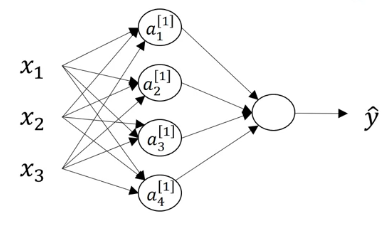
Imagine that you have a single training example $x$ with three features: $x_1, x_2, x_3$. Imagine also that you have a two layer neural network, that is a neural network with a single hidden unit. Finally also imagine that the hidden layer has $4$ hidden units $a^{[1]}_1, a^{[1]}_2, a^{[1]}_3, a^{[1]}_4$. 1
Now let’s focus on calculating $z^{[1]} = W^{[1]}x + b^{[1]}$. Notice that $W^{[1]}$ is a matrix and this is how it is built: remember that we have four hidden units in our hidden layer. This means that $z^{[1]}$ will have four elements, $z_1^{[1]}, z_2^{[1]}, z_3^{[1]}, z_4^{[1]}$, and this is how each of them is calculated:
- $z_1^{[1]} = w_1^{[1]T}x + b_1^{[1]}$
- $z_2^{[1]} = w_2^{[1]T}x + b_2^{[1]}$
- $z_3^{[1]} = w_3^{[1]T}x + b_3^{[1]}$
- $z_4^{[1]} = w_4^{[1]T}x + b_4^{[1]}$
Notice that $w_i^{[1]T}$ is actually a vector! Its size is the size of the previous layer, your features, so each $w_i^{[1]T}$ has three elements, each of which is multiplied by each of your input features. The main idea is to stack $w_i^{[1]T}$ into a matrix $W^{[1]}$, like this:
$$ \begin{equation} W^{[1]} = \begin{bmatrix} — & w_1^{[1]T} & — \\ — & w_2^{[1]T} & — \\ — & w_3^{[1]T} & — \\ — & w_4^{[1]T} & — \\ \end{bmatrix} \end{equation} $$
Remember that each $w_i^{[1]T}$ was of size 3, so our matrix $W^{[1]}$ is of dimensions $(4, 3)$. Because of how matrix-vector multiplication works when you define a vector as a column matrix, now we can do the whole thing in a single step. So that:
$$ \begin{equation} z^{[1]} = \begin{bmatrix} — & w_1^{[1]T} & — \\ — & w_2^{[1]T} & — \\ — & w_3^{[1]T} & — \\ — & w_4^{[1]T} & — \\ \end{bmatrix} \begin{bmatrix} x_1 \\ x_2 \\ x_3 \end{bmatrix} + \begin{bmatrix} b_1^{[1]} \\ b_2^{[1]} \\ b_3^{[1]} \\ b_4^{[1]} \end{bmatrix} = \begin{bmatrix} w_1^{[1]T}x + b_1^{[1]} \\ w_2^{[1]T}x + b_2^{[1]} \\ w_3^{[1]T}x + b_3^{[1]} \\ w_4^{[1]T}x + b_4^{[1]} \end{bmatrix} = \begin{bmatrix} z_1^{[1]} \\ z_2^{[1]} \\ z_3^{[1]} \\ z_4^{[1]} \end{bmatrix} \end{equation} $$
Which you can simply rewrite as:
$$ \begin{equation} z^{[1]} = W^{[1]}x + b^{[1]} \end{equation} $$
Which is a lot better!
Now let’s not forget about $a^{[1]} = \sigma(z^{[1]})$. This means that the sigmoid function $\sigma(x)$ is applied element-wise to $z^{[1]}$. So that:
$$ \begin{equation} a^{[1]} = \begin{bmatrix} \sigma(z_1^{[1]}) \\ \sigma(z_2^{[1]}) \\ \sigma(z_3^{[1]}) \\ \sigma(z_4^{[1]}) \\ \end{bmatrix} \end{equation} $$
Now let’s keep track of the dimensions. Remember that we have $1$ training example with $3$ features and our single hidden layer has $4$ nodes:
- $\underset{(4, 1)}{z^{[1]}} = \underset{(4, 3)}{W^{[1]}}\underset{(3, 1)}{x} + \underset{(4, 1)}{b^{[1]}}$
- $\underset{(4, 1)}{a^{[1]}} = \underset{(4, 1)}{\sigma(z^{[1]})}$
- $\underset{(1, 1)}{z^{[2]}} = \underset{(1, 4)}{W^{[2]}}\underset{(4, 1)}{a^{[1]}} + \underset{(1, 1)}{b^{[2]}}$
- $\underset{(1, 1)}{a^{[2]}} = \underset{(1, 1)}{z^{[2]}}$
Notice that the dimensions of the arrays are below them. Remember that the product $AB$ of two matrices $A, B$ is only defined if the number of columns in $A$ equals the number of rows in $B$. So that you can multiply a $m \times n$ matrix $A$ by a $n \times p$ matrix $B$, and the result $AB$ will be a $m \times p$ matrix. This is exactly why the dimensions have to line up. 2
Vectorizing across multiple examples
Previously, $x$ was a single training sample. It had three features so that $x \in \mathbb{R}^3$ (this means that $x$ belongs to the set of all vectors that live in three-dimensional space).
We could run a for loop for each of our training samples and do the calculation in the previous section for each of the elements, but it turns out that linear algebra is the gift that keeps on givin'.
If we stack our training samples $x_1, \dots x_m$ as columns of a matrix $X$ we can make our life infinitely easier. If our data has $n$ feature and $m$ training examples, then:
$$ \begin{equation} \underset{(n, m)}{X} = \begin{bmatrix} \mid & \mid & & \mid \\ x^{(1)} & x^{(2)} & \dots & x^{(m)} \\ \mid & \mid & & \mid \\ \end{bmatrix} \end{equation} $$
Notice that $x_i$ refers to the $i$th feature of a training example, while $x^{(i)}$ refers to the $i$th training example.
Now we can rewrite our neural net with matrices for $Z^{[l]}, A^{[l]}$:
- $Z^{[1]} = W^{[1]}X + b^{[1]}$
- $A^{[1]} = \sigma(Z^{[1]})$
- $Z^{[2]} = W^{[2]}A^{[1]} + b^{[2]}$
- $A^{[2]} = \sigma(Z^{[2]})$
Similar to how the training examples are stacked in the columns of $X$, each training example is a column of $A^{[l]}, Z^{[l]}$. In the case of $A^{[k]}$, the entry $i, j$ corresponds to the $i$th hidden-unit’s activation of the $k$th hidden layer on the $j$th training example.
On a personal note, I think that Andrew’s explanation of this is exceptional, and highlights the importance of being able to abstract away from one-training-example scale to neural-network scale.
Activation functions
So far we’ve picked the sigmoid function, $\sigma(x)$, and slapped it at the end of our linear regression. But why did we pick it? We picked it to add non-linearities, which are important to deal with datasets that are non-linearly separable. Also think that the composition of two linear functions is itself a linear function. Without any non-linearities your network would not be able to learn more “interesting” (non-linear) features as you go deeper in the layers. It turns out however, that this is not our only choice, and in fact the choice matters in many ways.
Tamara Broderick is an Associate Professor at MIT, where she teaches machine learning and statistics. Being an all-around amazing person, she has published an entire course of machine learning on YouTube, and the slides made public on her website. The reason I mention this, besides the fact that she is an amazing teacher, is that her slides are beautiful; geometrically so. In her slides, you can see why how the choice of activation function changes the decision plane in graphical detail. I 100% suggest you check out these slides and marvel at the geometric beauty of neural nets!
It turns out that there are three widely used (some more than others) activation functions. We denote the activation function of layer $l$ as $g^{[l]}$. The functions are:
- Hyperbolic Tangent Function: $g^{[l]}(z^{[l]}) = \text{tanh}(z^{[l]}) = \frac{e^z - e^{-z}}{e^z + e^{-z}}$
- Standard Logistic Function: $g^{[l]}(z^{[l]}) = \sigma(z^{[l]}) = \frac{1}{1 + e^{-z}}$
- Rectified Linear Unit (ReLU): $g^{[l]}(z^{[l]}) = \text{ReLu}(z^{[l]}) = \max(0, z)$
Now when do you use which? Only use the $\sigma(z)$ as your output function. If your output is strictly greater than $0$, you could also use a $\text{ReLU}(z)$ here as well, even for regression. Sometimes you don’t need a non-linear activation function in your output layer for regression. The $\text{tanh}(z)$ function is strictly superior to $\sigma(z)$ in hidden layers. Most commonly use the $\text{ReLU}(z)$ in hidden layers. Why? Because of differentiation! The derivatives of these functions have to be well-behaved across the domain in order for our fancy gradient descent to not get bogged by numerical precision issues. This is later covered in the course under the name of exploding or vanishing gradients.
Random Initialization
How do we initialize our parameters? The choice of how we initialize our $W^{[l]}$ actually matters. There is a property known as symmetry. If you choose all your parameters as $0$, then you are not “breaking” symmetry. What this means is that every iteration of gradient descent will result in the same weights, therefore it will never improve your cost. You might be asking, hey what about $b^{[l]}$? It turns out that $b^{[l]}$ doesn’t have the symmetry problem, so you don’t need to worry too much about it, and can in fact initialize it to $0$.
Fine, but what do we initialize it to? You can use random numbers (actually not just any random numbers as we will see in the next course), with the only caveat that you need to scale your randomly chosen parameters by a constant, usually $0.01$ or $10^{-2}$. This is done to keep the numbers close to $0$, where the derivatives of your activation functions are better defined than at the extremes. Remember that $\sigma(z^{[l]})$ is basically flat for values $|x| \approx 6$. There are more sophisticated approaches to parameter initialization that will are covered in the next course.
Next week’s post is here.
Deep Learning Specialization | Coursera, Andrew Ng ↩︎