This is the third and final week of the second course of DeepLearning.AI’s Deep Learning Specialization offered on Coursera.
This week’s topics are:
Hyperparameter Tuning
We have seen by now that neural networks have a lot of hyperparameters. Remember that hyperparameters remain fixed during training. This means that the process of finding reasonable hyperparameters, called hyperparameter tuning, is a process that is separate from training your model.
Tuning Process
As mentioned above, neural networks can have a lot of parameters:
- $\alpha$: the learning rate.
- $\beta$: the EWMA term in momentum.
- $\beta_1, \beta_2, \epsilon$: the EWMA parameters for Adam.
- The number of layers $L$.
- The number of hidden units $n^{[l]}$.
- Learning rate decay rate if using learning rate decay.
- The size of mini batches.
If it seems daunting, it’s because it is. Hyperparameter tuning is necessary most of the time because good hyperparameters from one problem not always translate to other problems. However, there are some hyperparameters that are usually more important than others. This can help you guide your tuning to focus on the most important ones first.
In the course, Andrew defines three tiers of importance for hyperparameter tuning, the first ones being more important than the latter ones:
- $\alpha$
- $\beta$ if using momentum. Using $\beta = 0.9$ is a good default. The number of hidden layers and the mini-batch size.
- Learning rate decay, and $L$.
If using Adam the defaults of $\beta_1 = 0.9, \beta_2 = 0.999, \epsilon=10^{-8}$ usually work fine.
Now we know where to focus first. But how do we actually search and evaluate values?
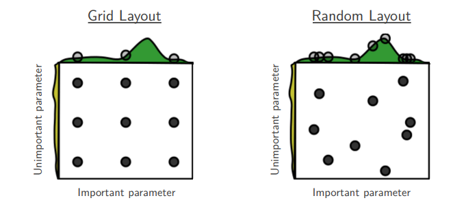
In the earlier generation of machine learning algorithms, researchers would usually use grid search. Grid search is an exhaustive search over a manually specified subset of the hyperparameter space, usually using cross validation. It’s called a grid because if you imagine having two hyperparameters $h_1, h_2$, and some range of values and a step-size for each of the ranges $r_1, r_2$, then you can imagine a grid or matrix where each cell is a combination of $h_1, h_2$ over each of their ranges. For example, you might say, I want to search a value for $\alpha$ in the interval $[0.001, 0.1]$, and I will draw some equidistant samples in that range and evaluate all the values. Notice that the “grid” becomes a matrix, or $n$-dimensional tensor as you add more hyperparameters; this is terrible because the volume of the search space increases exponentially with each additional dimension or hyperparameter.
Random Search
Staying within the simple example of using two hyperparameters $h_1, h_2$, the problem with grid search might be apparent: you evaluate the same value for each hyperparameter multiple times. If set a grid of $9$ cells, then each value of both $h_1, h_2$ will be tested three times while holding the other constant. This is why the recommendation is to use random search: where each combination of $h_1, h_2$ is unique (the probability of repetition being low if you sample appropriately at random). The following image illustrates this point:
Coarse-to-fine Grained Search
Another, optional, recommendation is to first find a promising range for search and then zoom in within the range. This is called coarse-to-fine grained search.
Using an Appropriate Scale when Searching
So we know that we should sample the hyperparameter space at random. However, this doesn’t necessarily mean to do it uniformly at random. The reason for this is that the search scale for each hyperparameter matters a lot. Being able to communicate the desired scale to the random sampling process is crucial for efficient search.
For some hyperparameters, such as the size of a hidden-layer $l$, $n^{[l]}$, it might be reasonable to sample uniformly at random. Say that you want to search for $n^{[l]}$ over the range $[50, 100]$. Then values like $89, 57, 62, 89, 74$ might be reasonable (actually sampled at random).
Remember that a continuous uniform distribution has a PDF of $\frac{1}{b-a}$ where $a,b$ are the minimum and maximum values. Therefore, every value in the range $[a, b]$ has the same probability of being realized.
This will not work for a hyperparameter like $\alpha$, however. Say that we suspect that a good $\alpha$ value is in the range $[0.0001, 1]$, and we sample uniformly at random. Since every value has the same likelihood of being drawn, this means that values between $[0.1, 1]$ will be sampled with $90\%$ probability. What about the interval $[0.0001, 0.1)$? These values have only a $10\%$ probability of being drawn. This is terrible because we are equally interested in values in both ranges.
This is why it makes more sense to sample for $\alpha$ values on the log scale as opposed to the linear scale. When we search over the linear scale and sample uniformly at random, we will spend $10\%$ of our effort searching over $[0.0001, 0.1)$ and $90\%$ of our effort searching over $[0.1, 1]$. On the other hand, when using a log-scale and sampling uniformly at random, we will spend an equal amount of effort searching over $[0.0001, 0.001), [0.001, 0.01), [0.01, 0.1), [0.1, 1]$.
Python Implementation
The way to implement the example above is as follows on Python:
np.random.seed(1337)
r = -4 * np.random.rand()
print(10 ** r)
0.0895161303335359
Let’s break this down. Remember that np.random.rand() generates random samples from a uniform distribution over the interval $[0, 1]$. Now, when we want to sample uniformly at random on a log scale, we want to sample uniformly in the exponents. What exponents? In our case, we want to sample uniformly in the range of $[0.0001, 1]$ which is the same as $[10^{-4}, 10^{0}]$. So if we can draw random samples $r$ from a uniform random distribution in the range $[-4, 0]$, then we can plug those into $10^{-r}$ and thus generate the samples in the log scale. How do we get $-4$? It’s as simple as $-4 = \log_{10}0.0001$.
Let’s generate $10$ such values for $\alpha$ in a vectorized way:
np.random.seed(1337)
rs = -4 * np.random.rand(10)  # we draw 10 samples
print(10 ** rs)  # this is vectorized over `rs`
array([2.31880438e-01, 7.71780714e-02, 1.45456272e-02, 5.19993408e-02,
       8.44167674e-03, 8.95835560e-02, 1.24640408e-04, 1.17149864e-03,
       3.45862195e-01, 2.85036007e-02])
Hyperparameter Tuning in Practice: Pandas vs. Caviar
Andrew mentions that there are two ways that hyperparameter tuning happens in practice: pandas vs. caviar. No, it’s not related to the pandas Python package. It’s related to how the animal, the giant panda, has offspring. Pandas usually have very few offspring and therefore put a lot of effort into the upbringing of each (don’t think too heavily on the veracity of this statement). This is contrasted to other species that lay thousands of eggs, where each egg is almost left to chance (again no offense to the regal Giant Pacific Octopus mothers whom sometimes give their lives for their precious 120,000 to 400,000 eggs).
The idea is that sometimes your model is too big, and you cannot afford to train multiple instances of your model, so must babysit it like a little panda. That is, adjusting the hyperparameters over longer periods of time. On the other hand, the caviar approach is where you can afford to train multiple models in parallel with different hyperparameters and then pick the winner.
Batch Normalization
You might remember how we mentioned that normalizing your inputs could help our optimization run faster. The issue with this is that even though our input layer is getting normalized values, the outputs of each layer $l$, $A^{[l]}$ are no longer normalized. Batch normalization is applying the same reasoning but on each layer.
Batch normalization doesn’t have anything to do with batch or mini-batch gradient descent and can be implemented under both approaches.
A key thing is that we won’t normalize $A^{[l]}$ but $Z^{[l]}$ instead. Let’s go over the steps.
Normalizing Activations in a Network
For a given layer $l$ in our network, under the batch gradient descent approach, we compute:
$$ \begin{equation} Z^{[l]} = W^{[l]}A^{[l-1]} + b^{[l]} \end{equation} $$
Now, we will normalize $Z^{[l]}$ via standardization:
$$ \begin{equation} Z^{[l]}_{norm} = \frac{Z^{[l]} - \bar{Z}^{[l]}}{S^{[l]} + \epsilon} \end{equation} $$
Where $\bar{Z}^{[l]}$ is the sample mean of $Z^{[l]}$ and $S^{[l]}$ is the sample standard deviation of $Z^{[l]}$.
Finally, we compute $\tilde{Z}^{[l]}$ by:
$$ \begin{equation} \tilde{Z}^{[l]} = \gamma^{[l]} Z^{[l]}_{norm} + \beta^{[l]} \end{equation} $$
There should be nothing new until the last step; we just standardized $Z^{[l]}$. But what is this new $\tilde{Z}^{[l]}$? It’s simply a rescaled and re-shifted version of $Z_{norm}^{[l]}$. Remember that standardizing samples of random variable will make them have approximately mean $0$ and variance $1$ if the random variable is normally distributed. Maybe this particular center and spread is not what’s best for our model. Remember what happens in regularization when $Z_i^{[l]} \approx 0, \forall i$ and $g^{[l]} = \sigma(x)$; maybe centering our $Z^{[l]}$ around $0$ makes our neural network approximately linear.
Having $\gamma^{[l]}, \beta^{[l]}$ allows us to shift and scale $Z^{[l]}_{norm}$ in a way that improves the performance of our model. Yes, this means that $\gamma^{[l]}, \beta^{[l]}$ are new parameters that we can learn via our garden variety gradient descent.
Think about what happens when $\gamma^{[l]} = S^{[l]} + \epsilon$ and $\beta^{[l]} = \bar{Z}^{[l]}$. In this case the last step undoes the normalization! This is not relevant to the actual implementation but simply to highlight that the learnable parameters are as powerful as standardizing.
Fitting Batch Norm into a Neural Network
So now we have $\gamma^{[l]}, \beta^{[l]}$ for each of our hidden layers $l$. Remember that $\beta^{[l]}$ is different from $b^{[l]}$ and also different from the $\beta$ parameter used in gradient descent with momentum. We can learn these parameters in the same way we have been learning $W^{[l]}, b^{[l]}$; that is updating them on each step of gradient descent. We can even use EWMA methods such as momentum, RMSProp or Adam. One of the amazing things about these approaches is that they’re generalizable.
When using mini-batch gradient descent, we use the mean and standard deviation of each mini-batch to standardize. However, the $\gamma^{[l]}, \beta^{[l]}$ is the same for all mini-batches within a layer $l$.
A final detail mentioned in the course is that, when using batch normalization, the parameters $b^{[l]}$ are redundant because they are subtracted when standardizing. Therefore, you can drop $b^{[l]}, \forall l$ from the set of learnable parameters and simply focus on $\beta^{[l]}$.
Why does Batch Norm work?
Earlier we discussed how normalization helps the optimization by undoing weird scales in our data. Batch norm works on the exact principle, but not just on the input layer; it applies this idea to all the layers. Remember that the hidden-layers are the “feature generation” layers, so this also means that batch norm undoes any weird scaling issues produced by layer $l-1$ which affect layer $l$, but also layer $l+1$ and so on.
Another way to think about this is to think about what happens in the following scenario. Imagine that we train a cat classifier using only cat pictures of cats with black fur. Assuming that our classifier performs well, it might not perform well on tasks where cats are allowed to have different fur colors than black. This is called covariate shift, and it simply means that our training data comes from a different distribution than the testing data. What batch norm does it to weaken the coupling between layer $l$ and layers $1, 2, \dots, l$, which can be thought of as internal covariate shift.
Finally, batch norm can act as a slight regularization. This occurs because when using batch norm with mini-batches, there is sampling error in the estimates of the mean and variance of each mini-batch. This noise ends up having a similar effect to dropout, which can result in some slight regularization. The noise added is inversely proportional to the mini-batch size by $O\left(\frac{1}{\sqrt{n}}\right)$, so that the larger the mini-batch size the less the regularization effect.
Batch Norm at Test Time
When we train our network with mini-batch batch norm, we calculate the mean and variance within each mini-batch. What happens when we want to make predictions or test our model? How can we calculate the mean and variance for a single test example?
We don’t. Instead, we keep a running average of the mean and variance for each layer using our favorite EWMA method during training. The last value is the one we use for testing, that is, the latest EWMA estimates for each layer’s mean and variance.
Andrew also mentions that batch norm is pretty robust to the particular approach you use to estimate the mean and variance when testing time. If you estimate it using your entire training set or if you use an EWMA approach, the results should be very similar.
Multi-class Classification
Softmax Regression
So far, all classification examples have been for binary classifiers, i.e. we only have two classes to predict: is this cat or not? What happens when we want to classify many classes, such as cats, dogs, baby chicks and anything else?
We denote the number of classes as $C$. In the case above $C = 4$. Ideally we want to go from an input image, to a vector $A^{[L]} = \hat{y}$, where $\hat{y}_1 = P(C_1 \mid x), \hat{y}_2 = P(C_2 | x), \dots, \hat{y}_k = P(C_k | x)$. That is, each entry in $\hat{y}$ describes the probability that an input $x$ belongs to each class $k \in C$. Since each class should be independent, it would be nice if:
$$\sum_{i=1}^k \hat{y}_k = 1$$
That is, the probabilities for each class should add up to one, that being one of the requirements of a valid sample space. We solved this in the binary case using our trusty old friend the sigmoid $\sigma(x)$, which maps $\mathbb{R} \rightarrow (0, 1)$. But the sigmoid $\sigma(x)$ takes a single scalar, what can we do if $x$ is a vector? That is, what can we do when we have more than 2 classes? It turns out that there is a generalization of the sigmoid $\sigma(x)$ called the softmax function.
The standard (unit) softmax function $\sigma: \mathbb{R}^K \mapsto (0, 1)^K$. This means that the softmax function $\sigma$ maps a $K$ dimensional real-valued vector, to a $K$ dimensional vector where each element is in the interval $(0 ,1)$, and it’s defined when $K \geq 1$ by:
$$ \begin{equation} \sigma(\mathbf{z})_i = \frac{e^{z_i}}{\sum_{j=1}^K e^{z_j}} \end{equation} $$
Notice that in our case, $K = C$ where $C$ is the number of classes in our approach. Notice that because of the denominator, which is normalizing, all of our values will add up to $1$, which is exactly what we want.
Let’s walk over one example. Assume that:
$$ \begin{equation} Z^{[l]} = \begin{bmatrix} 5 \\ 2 \\ -1 \\ 3 \end{bmatrix} \end{equation} $$
Now let’s calculate $A^{[l]} = \sigma(Z^{[l]})$ using the softmax. We will do this in two steps, first calculate the numerator, $t$:
$$ \begin{equation} t^{[l]} = \exp(Z^{[l]}) = \begin{bmatrix} e^5 \\ e^2 \\ e^{-1} \\ e^3 \end{bmatrix} = \begin{bmatrix} 148.4 \\ 7.4 \\ 0.4 \\ 20.1 \end{bmatrix} \end{equation} $$
Now we normalize $t^{[l]}$ by the sum $\sum_{j=1}^4 e^{t_j} = 176.3$ to get $A^{[l]}$
$$ \begin{equation} A^{[l]} = \hat{y} = \frac{t^{[l]}}{176.3} = \begin{bmatrix} \frac{148.4}{176.3} \\ \frac{7.4}{176.3} \\ \frac{0.4}{176.3} \\ \frac{20.1}{176.3} \end{bmatrix} = \begin{bmatrix} 0.842 \\ 0.042 \\ 0.002 \\ 0.114 \end{bmatrix} \end{equation} $$
Now we can interpret these as probabilities! For example $P(x | C_1) = 0.842, P(x | C_2) = 0.042$ and so on. Also notice that the sum of these is $1$ because of the normalization in the denominator. Of course, we can think of the softmax as just another activation function, albeit a multi-dimensional one.
The name softmax comes from the comparison against the “hard max” function, which used in our case would return the vector $[1, 0, 0, 0]$, that is a boolean mask of the maximum value in the vector. The softmax is a “continuous” or “soft” version of that so that the vector we get as output is $[0.842, 0.042, 0.002, 0.114]$.
You might be thinking, what if $C=2$? In this case we are back to binary classification. If we compare softmax regression to logistic regression, then when $C=2$ softmax reduces to logistic regression. However, softmax can generalize logistic regression to $C=K$ dimensions or classes.
Training a Softmax Classifier
It turns out that using negative log loss as your loss function generalizes nicely to many classes, i.e. $C > 2$.
Another thing to keep in mind if we are using the vectorized implementation, where:
$$ Y = [y^{(1)}, y^{(2)}, \dots, y^{(m)}] $$
Then both $Y$ and $\hat{Y}$’s dimensions will be $(C, m)$ now instead. That is each sample $m$ will have it’s own softmax vector describing the probability that it belongs to each class.
Programming Frameworks
Okay, never program your deep learning framework from scratch unless you are an expert trying to squeeze the latest bits of performance in some kind of specialized hardware. Just go with your favorite deep learning framework package. Hopefully go with one that has a vibrant, active community where you can get support and learn how to use the framework.
Most of the frameworks differ in their approaches and they ultimately end up being equivalent. Like many other packages, measuring the “best” is hard because the “best” package is not just the fastest, but the easiest to use, the one with the best community and support, etc.
The key thing that all frameworks share is that they solve the problem of automatic differentiation. That is you can define some data, some kind of optimizer, some kind of cost function, and then automatically differentiate the cost function with respect to some parameters. For the purposes of the course, all frameworks should be thought of as equivalent. The course goes over a very simple TensorFlow example, but I decided to ignore it since TensorFlow’s documentation has better introductory examples in my opinion.
Next week’s post is here.