Improving Deep Learning Networks: Week 1 | Practical Aspects of Deep Learning

This is the first week in the second course of DeepLearning.AI’s Deep Learning Specialization offered on Coursera. The course deals with hyperparameter tuning, regularization and the optimization of the training process. The optimization ranges from computational complexity to performance. This is again a pretty technical week, where you will benefit a lot from doing the programming exercises.

This week’s topics are:

Setting up our Machine Learning problem
Regularizing our Neural Network
Setting up our Optimization Problem
Normalizing Inputs
Vanishing and Exploding Gradients
Weight Initialization

Setting up our Machine Learning problem Link to heading

Train / Dev / Test sets Link to heading

Machine learning projects are highly iterative. That is, you try something new, see how it does and then adjust; very much like gradient descent. Therefore, you want the iteration time to be quick so that you can try as many things as quickly as possible, without affecting the final performance of the model. Part of this is setting up your datasets correctly so that you can efficiently iterate over different approaches.

If you have a data set $M$ of $|m|$ samples then you usually want to split it into three parts.

Training set: $M_{train} \subseteq M$. The set of samples that will be used to learn the parameters of our chosen hypothesis $h(X, \theta)$, i.e. your model parameters via SGD.
Holdout/Cross-validation/Development set: $M_{dev} \subseteq M$. The set of samples that will be used to evaluate a hypothesis class $H$, i.e. your model hyperparameters via hyperparameter tuning.
Test set: $M_{test} \subseteq M$. The set of samples that will be used the best hypothesis you’ve found so far on completely unseen data that belongs to the same distribution as the dev set.

Note that these three subsets are disjoint, i.e. $M_{train} \cap M_{test} \cap M_{dev} = \emptyset$

Historically most researchers would split the set $M$ using a 70%/30% training and testing respectively. If using a dev set, a 60%/20%/20% split for training, dev and test. This was reasonable for datasets that have sizes in the order of 10,000. If you have a dataset $M$ with 1,000,000 training samples, then it can be reasonable to use a 98%/1%/1% training, dev and test split. You can read more about how big a sample has to be for certain statistical properties to kick in, but a number around 10,000 is considered relatively safe.

One assumption is that all the training samples $m \in M$ come from the same distribution, which implies that each of the splits also belong to the same distribution. This is critical because you don’t want to develop a model with pictures of cats and then test it on picture of dogs. A key thing is to make sure that your dev and test sets come from the same distribution. Having the training set come from a different distribution is more lax, as long as the training distribution is a superset of the dev and test sets. In some cases it might be okay to not have a test set, but measuring variance will be harder.

Bias-Variance Tradeoff Link to heading

The bias/variance tradeoff is a topic in machine learning and statistics. The whole idea of supervised learning is that, if you do it correctly, your model can generalize beyond the training set, i.e. samples it has not seen during training and still do a good job. We think that there are some parameters $\theta$ that minimize our cost function. We don’t know what that is, and the only way to know that is to have infinite training samples. But we need to make due with our estimate $\hat{\theta}$, which implies that $\theta \neq \hat{\theta}$. When we talk about the bias-variance tradeoff we are describing the errors, i.e. $\epsilon = \theta - \hat{\theta}$ that are produced by our model that uses our estimates of the parameters. In particular, we are describing the mean and variance of the error distribution. The bias is a part of how far $\hat{\theta}$ is from $\theta$ on average, while the variance measures the spread of the errors.

It turns out that we can characterize our expected test errors even further by decomposing them into three components (skipping some math):

Variance: $E_{x, D}\left[\left(h_D(x) - \bar{h}(x)\right)^2\right]$
$\text{Bias}^2$: $E_x\left[\left(\bar{h}(x) - \bar{y}(x)\right)^2\right]$
Noise: $E_{x,y}\left[\left(\bar{y}(x) - y\right)^2\right]$

Keep in mind:

Variance measures how much our classifier $h_D$ changes when we train it on a different training set $D$. How “over-specialized” is our classifier to a particular training set $D$? ¹ Notice that $h$ and $h_D$ are random variables, and so this measures the spread of a classifier trained on each possible sample $D$ drawn from $P^n$ versus the average classifier $\bar{h}(x)$.
Bias measures the inherent error from our classifier if we had infinite training data. ¹ How far is our estimator’s expected value $\bar{y}(x)$ from the expected classifier?
Noise measures some irreducible error, which is an intrinsic property of the data. This related to Bayes error rate, which is the lowest possible error rate for any classifier of random outcomes.

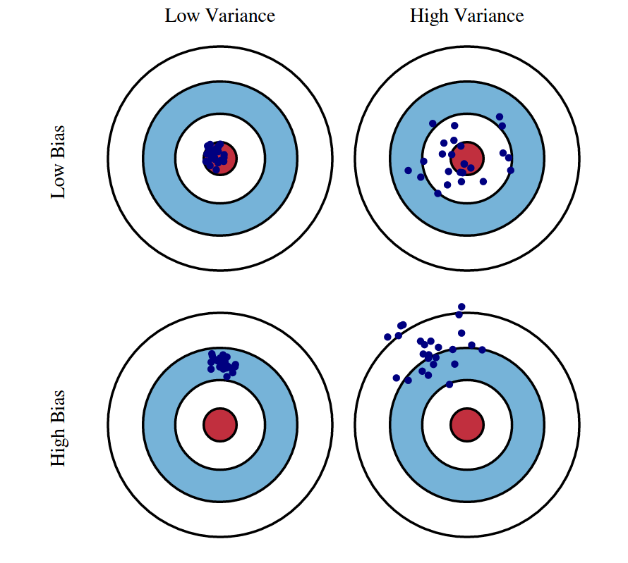
Graphical Illustration of bias and variance

We know that bias and variance are the components of our model’s expected test error. But why is it a tradeoff? It turns out that model complexity is related to both bias and variance. A model with low complexity (always guess the same) will have high error, and the majority of the error will come from the bias term. This means that as we decrease the complexity of a model, our error will increase, but most of the increase will come from the bias term. Conversely, a model with high complexity (guessing randomly) will have high error, and the majority of the error will come from the variance term. This means that as we increase model complexity, our error will also increase, but most the increase will come from the variance term. Somewhere in the middle, there is a sweet spot, a combination of bias and variance that has the minimum total error.

When we say that a model has high bias, we say that it’s underfitting. It’s too basic and not being complex enough to learn the training data, underfitting it. On the other hand, when we say that a model has high variance we say that a model is overfitting the training data, not being able to generalize beyond it, overfitting it. This is where we come back to our dataset splits.

Before moving on, we have to re-introduce the irreducible error term from the previous section. For every classification task, there is some amount of error that cannot be done away with. This is also called Bayes error rate, and it’s a theoretical limit that no classifier can surpass. Similarly, there is a human-level error achieved by the best a human can do, whether a group or individual, and this is called the human-level error. The best classifier can be better or worse than human-level error but never better than Bayes error rate. For the following section we assume that the human-level error is approximately $0$ but more than the Bayes error rate.

Evaluating the performance of your model on the training and dev set can help you diagnose whether your model has high variance or high bias or both very quickly. Let $\epsilon_{train}, \epsilon_{dev}$ the error of your model on the training and dev sets respectively.

$e_{train} = 1\%, e_{dev} = 11\%$: Our model is doing really well on the training set but much poorer on the development set. It smells of high variance since the model is not able to generalize from the training set to the dev set. It’s therefore overfitting the training set.
$e_{train} = 15\%, e_{dev} = 16\%$: Assuming that human-level error is approximately $0$, then this looks like high bias. The model is very far from human-level error on the training set, therefore it’s not fitting our training data enough. It’s therefore underfitting the training set. However, it’s generalizing quite well to the dev set, therefore it might have low variance.
$e_{train} = 15\%, e_{dev} = 30\%$: Assuming that human-level error is approximately $0$, then this looks like high bias again. But because it’s not generalizing well, it also smells of high variance because of the discrepancy in performance between the test and dev sets.
$e_{train} = 0.5\%, e_{dev} = 1\%$: Assuming that human-level error is approximately $0$, then this looks like both low bias and low variance. It’s very close to the Bayes' error rate, and also generalizes well to the dev set.

The key assumption is that human-level error is approximately $0$, which implies that Bayes error has to be between $0$ and the human-level error. If for example the Bayes error rate is $15\%$ then the second case would not be high variance, because we are actually close to the best possible classifier.

If you’re wondering about how you can simultaneously underfit and overfit your training data, think about this:

Basic Recipe for Machine Learning Link to heading

Ideally we want a low-bias and low-variance model. But how do we get there?

Do we have high bias? How is our performance on the training set relative to Bayes error rate?
- If high bias:
  - Increase the size/depth of your network, adding model complexity, increasing variance but lowering bias.
  - Train it longer, better estimates of the parameters, lower bias and variance.
Do we have high variance? How is our performance on the dev set relative to the training set and Bayes error rate?
- Get more data, better estimates of the parameters, lower bias and variance.
- Regularization, decreasing model complexity, increasing bias but lowering variance.

Following these steps, i.e. fixing high bias before high variance is the basic recipe for machine learning.

It’s mentioned in the course that in the deep learning era, there is less of a tradeoff. The ability to have bigger models and get more data are both tools that don’t expose the bias-variance tradeoff, so usually these are the first things to check when encountering high bias or high variance. In general training a bigger network almost never hurts, as long as you add proper regularization, keeping the model complexity from exploding.

Regularizing our Neural Network Link to heading

Regularization Link to heading

Regularization is a tool you employ when you suspect your model is suffering from high variance or overfitting. Regularization will reduce your model complexity by penalizing model complexity when evaluating its performance and therefore generating a “simpler” model. It turns out that you can add a term to your cost function, which is a measure of model complexity, so that more complex models result in a higher cost, therefore driving down complexity. But how do we measure model complexity? Let’s answer this using the logistic regression case:

Let’s recall our cost function:

$$ \begin{equation} \mathcal{J}(w, b) = \frac{1}{m} \sum_{i = 1}^m \mathcal{L}(\hat{y}^{(i)}, y^{(i)}) \end{equation} $$

We would like to add something to the expression above that measures model complexity. One way of measuring model complexity is literally to look at the magnitude of the parameters, literally how big they are. Remember that in logistic regression we have one theta $\theta_i$ for each feature in our data. This implies that if coefficients blow up in magnitude, that is, get very big or very small, they are having a lot of effect on the output. This is simply because the relationship between parameters and features is multiplicative and additive, i.e. it’s linear.

We can check how big the parameters are by summing over each of them, let’s call that $|w|$:

$$ \begin{equation} |w| = \sum_{j=1}^{N_x} w_j \end{equation} $$

The issue with the above is that some $w_j$ might be positive and others might be negative, undoing each of their effects in the summation. The solution to this problem is to use a norm. A norm is a function that maps the real or complex numbers into the non-negative real numbers. An important geometrical idea related to linear algebra is that the norm is a generalization of distance from the origin: it’s proportional to scaling, it doesn’t violate a form of the triangle inequality, and is zero only at the origin. ² We would also like to generalize this to more dimensions, which is handy when our parameters is not just a vector but matrices that describe some vector space that has some “size”. When talking about the norm of a matrix, the term Matrix norm is used, and the euclidean norm equivalent is called the Frobenius norm. It has a different name because you have to do some work before generalizing from one to many dimensions and some brilliant mathematicians figured it out.

One of the most common norms is to take the squares to only get positive numbers. This is called the L2 Norm, or Euclidean norm for being related the definition of distance in Euclidean geometry, remember the guy Pythagoras?. It’s denoted $||w||_2$. When working with the square of the L2 norm, its denoted $||w||_2^2$. It’s defined by:

$$ ||w||_2 = \sqrt{\sum_{j=1}^{N_x} w_j^2} = \sqrt{w^Tw} $$

Also:

$$ ||w||^2_2 = w^Tw $$

Adding this to our cost function makes it looks like this now:

$$ \begin{equation} \mathcal{J}(w, b) = \frac{1}{m} \sum_{i = 1}^m \mathcal{L}(\hat{y}^{(i)}, y^{(i)}) + ||w||_2^2 \end{equation} $$

Why are we ignoring the other parameter $b$? Because it’s a scalar and not a vector. $w \in \mathbb{R}^{N_x}$, which means $w$ has $N_x$ elements. While $b \in \mathbb{R}$, which means that $b$ has only one element. This means that if we have $N_x$ features, then $b$ has to be $N_x$ times bigger than the $w$ norm to influence the same amount. You can also think about how the space or volume of a $N_x$ dimensional hypercube grows as opposed to a $1$ dimensional line. So we usually ignore $b$.

We now have a way of penalizing model complexity by assigning a higher cost to a more complex model. What would also be great is to have a way of scaling the effect of the regularization. For example, we don’t want a model with a very small $w$ because the smallest is where $w_i = 0$, we want to retain some complexity but not too much.

We do this by introducing a hyperparameter $\lambda$ called the regularization parameter, which is a scalar that scales the regularization effect:

$$ \begin{equation} \mathcal{J}(w, b) = \frac{1}{m} \sum_{i = 1}^m \mathcal{L}(\hat{y}^{(i)}, y^{(i)}) + \lambda||w||_2^2 \end{equation} $$

We can find a good $\lambda$ by hyperparameter tuning using the dev set. By comparing the loss between the training set and the dev set, we can find a good regularization value that balances simplicity and complexity, or bias and variance.

We also want to scale the effect of the regularization by the size of our training data $m$. Remember, we have a high variance problem we are trying to solve by penalizing a complex model. However, our model will be more complex as we add more training data. So we want our regularization to be stronger when our training data is small, but decrease as our training data is larger. We can just divide $\lambda$ by $m$ to have a linearly decreasing effect:

$$ \begin{equation} \mathcal{J}(w, b) = \frac{1}{m} \sum_{i = 1}^m \mathcal{L}(\hat{y}^{(i)}, y^{(i)}) + \frac{\lambda}{m}||w||_2^2 \end{equation} $$

Finally, for differentiation reasons, we add an easy way to cancel some terms:

$$ \begin{equation} \mathcal{J}(w, b) = \frac{1}{m} \sum_{i = 1}^m \mathcal{L}(\hat{y}^{(i)}, y^{(i)}) + \frac{\lambda}{2m}||w||_2^2 \end{equation} $$

Think about what happens to $w$ after we introduce this term to our cost function. It means it will prefer smaller parameters than bigger ones, and if it has to chose between two big ones, it will choose the one that is the least costly. In other words the model will let some parameters be large as long as they earn their keep (in terms of model performance) and decrease the features that are not that relevant. In this sense, regularization can be thought of as a type of feature selection. With the L2 norm the parameters that don’t earn their keep approach zero, but never quite get to be zero.

But the L2 norm is not the only norm. What if you use some other norm? Another popular norm is the L1-Norm:

$$ ||x||_1 = \sum_{j=1}^{N_x} |x_i| $$

Just like the L2-norm, it maps the real or complex numbers into the non-negative real numbers. We can also use this in our cost function:

$$ \begin{equation} \mathcal{J}(w, b) = \frac{1}{m} \sum_{i = 1}^m \mathcal{L}(\hat{y}^{(i)}, y^{(i)}) + \frac{\lambda}{2m}||w||_1 \end{equation} $$

Unlike the L2-norm, the L1-norm does actually send the parameters that don’t earn their keep to zero. This means that $w$ will end up being sparser. Which implies that the L1-norm works as a sort of model compression. In practice however, the L2 norm is used more commonly so that should be your first go to.

We mentioned the Frobenius norm as the generalization of the L2-norm to higher dimensions. The L2-norm works in logistic regression precisely because $w$ is a vector. When we have matrices of parameters, $W^{[l]}$ as is the case for a neural network, we need to use the grown-up’s norm. The Frobenius norm is a reasonable extension, instead of summing over a vector’s single dimension, you sum over both dimensions in a matrix:

$$ ||W^{[l]}||_F = \sqrt{\sum_{i=1}^{n^{[l - 1]}}\sum_{j=1}^{n^{[l]}}w_{ij}^{[l]}} $$

Also:

$$ ||W^{[l]}||^2_F = \sum_{i=1}^{n^{[l - 1]}}\sum_{j=1}^{n^{[l]}}w_{ij}^{[l]} $$

So for a $L$-layered neural network our cost function will look like:

$$ \begin{equation} \mathcal{J}(W^{[1]}, b^{[l]}, \dots, W^{[l]}, b{[l]}) = \frac{1}{m} \sum_{i = 1}^m \mathcal{L}(\hat{y}^{(i)}, y^{(i)}) + \frac{\lambda}{2m} \sum_{l=1}^L ||W^{[l]}||^2_F \end{equation} $$

A couple of things to mention:

Notice that now the cost function is a function of all layers of our network, $W^{[l]}, b^{[l]}$. This is in contrast to logistic regression where we only have one pair of $W, b$.
Also notice that in the regularization term we need to sum over all layers of our network. Again we are ignoring the $b^{[l]}$ and only focusing on the $W^{[l]}$ parameters.

The L2-norm is also usually called weight decay. This is because when you differentiate the loss function, which now includes the regularization term, with respect to the parameters, it will scale down $W^{[l]}$ by $1 - \frac{\alpha\lambda}{m}$ on every step. Making those weights smaller, or decaying the weights if you please.

If you’re coming from econ-land, you might have heard of Lasso and Ridge regressions. Lasso is a linear regression that uses the L1-norm, while Ridge is a linear regression that uses the L2-norm.

Why Does Regularization Reduce Overfitting? Link to heading

We went over how regularization is equivalent to penalizing model complexity, and how model complexity can be measured by the magnitude of the parameters of your model, which is the mechanism through which we implement regularization. The intuition here is that parameters with high values assign high sensitivity to the features being multiplied by those parameters. The high sensitivity is what results in the high variance, and by penalizing the magnitude of the parameters is how we reduce overfitting.

Another great way of thinking about it is to think about what happens in the activation functions when the values are big or small.

Remember that $Z^{[l]} = W^{[l]}A^{[l-1]} + b^{[l]}$. This, we pass through our activation function $g^{[l]}$ so that we get $A^{[l]} = g^{[l]}(Z^{[l]})$. Taking as an example the sigmoid activation function $\sigma(x)$, think about what happens when the inputs $Z^{[l]}$ are small. How can $Z^{[l]}$ be small? If we set $\lambda$ to be huge, then most of our $W^{[l]}$ will be small, therefore making $Z^{[l]}$ small as well. When we pass small values, that is values close to $0$ to the sigmoid function, the outputs are approximately linear. It is only when $|x| \geq 2$ that $\sigma(x)$ (approximately) becomes non-linear. So in a way, setting $W{[l]}$ to be small undoes all the non-linear magic that you got from adding more layers to your network.

Dropout Regularization Link to heading

It turns out that measuring the “size” of your parameters is not the only way to measure model complexity. Conversely, minimizing the size of your parameters is also not the only way to punish model complexity. Dropout achieves a similar result by doing something more intuitive to some.

In a nutshell, dropout randomly deletes some fraction of nodes in each hidden layer on each forward-backward pass. Since on each forward-backwards pass you are “turning off” some hidden units, the model trained on each iteration is literally smaller. The random component of the dropout guarantees that all parts of the model are affected equally on expectation. So what do we mean exactly by “deleting” nodes? We mean setting them to 0. It really is that simple.

More formally, there is some probability $p$ that represents probability for a single hidden unit to be kept untouched. $p$ is referred to as the keep probability. Conversely, $1 - p$ is the “dropout” probability. Notice that the events are independent of each other. That is each hidden unit, i.e. each node is dropped independently relative to all the other units in that layer, and also from other layers.

Say that you have a layer with $50$ hidden units, and that $p = 0.8$, so that you will be dropping out $1 - 0.8 = 0.2$ of the units in a hidden layer. So on expectation you will be dropping $50 * 0.2 = 10$ nodes. Let’s also think that this layer is $l = 3$. Let’s think about how this will affect the next layer.

The next layer’s computation will be:

$$ \begin{equation} Z^{[4]} = W^{[4]}A^{[3]} + b^{[4]} \end{equation} $$

Where $A^{[3]}$ is the output of the layer with $50$ hidden units, and we shut down $20\%$ of them. This means that $A^{[3]}$ is reduced by $20\%$, which also implies that $Z^{[4]}$ is reduced by $20\%$ because $Z^{[4]}$ is just a linear combination of $A^{[3]}$. In order to avoid this problem propagating throughout our network making everything small, we need to roughly “refund” the lost value to $A^{[3]}$ before passing it to the next layer. We do this simply by:

$$ \begin{equation} A^{[3]*} = \frac{A^{[3]}}{p} \end{equation} $$

Remember that dividing anything by a number less than $1$ will make it bigger. Therefore:

$$ \begin{equation} Z^{[4]} = W^{[4]}A^{[3]*} + b^{[4]} \end{equation} $$

Will make $Z^{[4]}$ be roughly the same as it was originally. This scaling technique is called inverted dropout.

The intuition behind this rescaling is that when you set some hidden-units to zero, you are shifting the expected value of $A^{[3]}$, which is an issue when you do testing. Because when you evaluate your network with the test set, you do not do any dropout, the difference in expected values becomes a problem. Therefore, the rescaling ameliorates the scaling issue between training and testing.

Finally, you can apply a different value of $p$ to different layers, so that you have a vector $p$ where $p^{[l]}$ is the probability of keeping units in hidden layer $l$. This faces you with a tradeoff of having more hyperparameters, so it should be used wisely.

Understanding Dropout Link to heading

So why does dropout behave like regularization? It seems crazy to “kill” some nodes at random, it’s the very definition of chaotic evil. It turns out that by doing this, the model will learn not to rely on any specific feature, because it might not be there the next time. The model will respond to dropout by spreading out the weights across the network, effectively reducing their magnitude. This is why dropout can be thought of as regularization.

An interesting approach to building resilience in engineering systems is that of Chaos Engineering. It’s similar in spirit to dropout, whereby randomly disabling some parts of a system, and forcing designers to deal with random failures will produce a more robust system.

Setting up our Optimization Problem Link to heading

One thing is to make sure that your model has the right combination of bias and variance, which amounts to learning the problem at hand well enough and also being able to generalize to unseen samples. Now, we turn our attention to making the optimization process (learning the problem) easier and more efficient.

Normalizing Inputs Link to heading

Normalization is one of those topics that means different things to different people. ³ Let’s disambiguate the term and also talk about why normalizing our inputs might be helpful for our optimization process.

As the name implies, normalization is the process of making something normal. Of course, there are many ways of making something “normal”, and we haven’t even defined what “normal” is. Let’s focus on one of the ways to normalize things.

In the context of statistics, normalization usually refers to standardizing, which is where we calculate a standard score for a random variable $X$. It’s called the standard score because its units are standard deviations.

Standardizing a random variable $X$ is pretty easy and intuitive:

$$ \begin{equation} z = \frac{x - \mu}{\sigma} \end{equation} $$

Where $\mu$ is the mean of the population and $\sigma$ is the standard deviation of the population. Because we don’t know those values, and we usually estimate them, we usually work with z-scores, which are the sample analogues:

$$ \begin{equation} z = \frac{x - \bar{x}}{S} \end{equation} $$

Where $\bar{x}$ is the sample mean and $S$ is the sample standard deviation. If your features are normally distributed, then the transformed variables will approximately mean zero and standard deviation of one.

The process is intuitive, for each observation we first ask: how far is this observation from the sample mean. Whatever that distance is, positive or negative, we scale it by the standard deviation. So that the result is: an observation is $z$ standard deviations from the mean.

But why do this? The purpose of this process is to convert different random variables that have different scales and shifts, into the same units. The units will be standard deviations for that particular random variable. So that $z_i$ will tell you how many standard deviations observation $i$ is from the mean. Positive values will be above the mean and negative values will be below the mean. Using this approach we can negate the effects of having different features with wildly different unit scales and shapes.

When you normalize your training set, you want to use standardization on each of your features separately. However, when you are testing, you want to use the same $\bar{x}$ and $S$ that you calculated during training. You don’t want to scale and shift your training data separately from your testing data. You want the opposite, you want your training and testing data to go through the same transformations.

How is this related to optimization? How does normalizing scales and shifts in our features affect our optimization? It all has to do with gradient descent and how the updates are made.

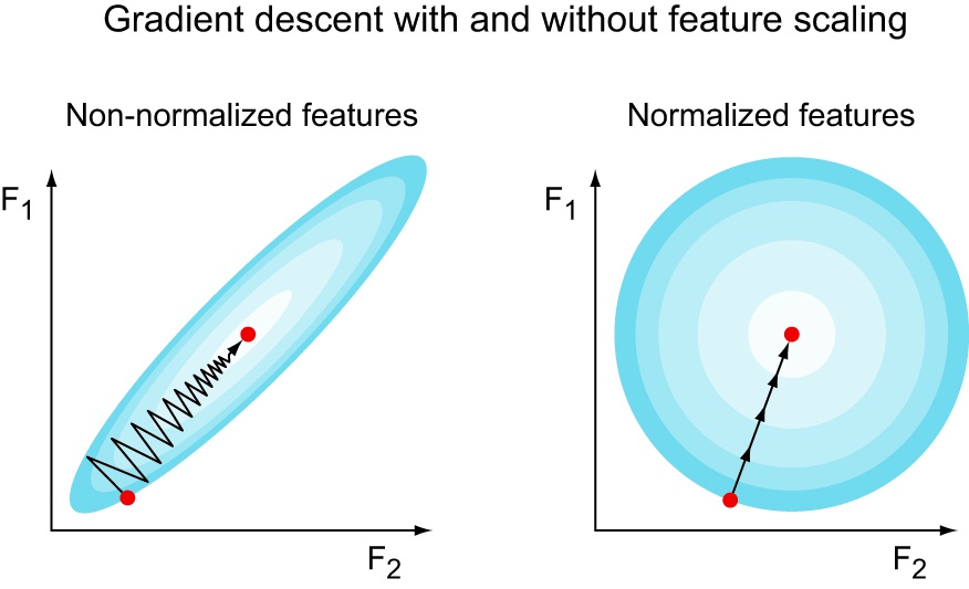
Gradient Descent with and without features scaling

The contour plot above shows an imaginary two-dimensional cost function $J(F_1, F_2)$. Notice that if we have a pair of unscaled features and one of the features' scale is larger than the other, then the cost function will look squished. Gradient descent will take many tiny steps because it’s considering both features at the same time. Since one feature is big and the other one small, the same step size is big in one but small on the other. This means that the larger feature will dominate the update. However, if you scale your features with standardization for example, then the cost function might look like the one on the right. Since all features are in a standard scale, no feature will dominate the update, allowing for less oscillation, and therefore faster convergence.

Vanishing and Exploding Gradients Link to heading

Vanishing and exploding gradients sound magical, if not outright dangerous. What this means is that when we train very deep networks, and we take the derivatives for gradient descent, the magnitude of these derivatives either “vanish” to $0$ or “explode” towards $\infty$. How does this disaster come about?

Think about a very deep $L$-layered neural network. Imagine also that all $W^{[l]}$ are the same:

$$ \begin{equation} W^{[l]} = \begin{bmatrix} 1.5 & 0 \\ 0 & 1.5 \end{bmatrix} \end{equation} $$

Also imagine that all $b^{[l]} = 0$.

Since all $W^{[l]}$ are the same, then whatever our features $x$ is, we get that:

$$ \hat{y} = W^{[l]L}x $$

That is the $W^{[l]}$ is multiplied by itself $L$ times. In our case this amounts to $1.5^L$, which literally grows exponentially with the number of layers. Imagine now that instead of $1.5$ on the diagonal of $W^{[l]}$ we have a number less than 0, i.e. $0.5$. With the same problem setup, now the values will be $0.5^L$ which is an expression that shrinks exponentially in the number of layers.

In either case, this is a huge problem. With exploding gradients, the gradient descent steps are gigantic, and with vanishing gradients the gradient descent steps are tiny. Either way, converging the minimum of our cost function will take a long, long time. We tackle this issue by being more careful in the way that we initialize our parameters.

Weight Initialization Link to heading

In order to avoid exploding or vanishing gradients, we need to be more careful as to how we initialize our parameters. The main idea here is that the more hidden units in a hidden-layer, the smaller each $w^{[l]}_j$ you want. This is to keep large hidden layers and small hidden layers in around the same output scale.

We will still initialize our parameters to random values, but we will scale them by a term, $s$, that is proportional to the size of the inputs coming into a layer $l$. The whole point of this is to adjust the variance of $W^{[l]}$ so that it’s proportional to inputs, $n^{[l-1]}$:

$$ \begin{equation} W^{[l]} = \texttt{np.random.randn(shape)} \times s \end{equation} $$

The choice is $s$ depends on $g^{[l]}(x)$, the activation function for layer $l$:

In the case that $g^{[l]}(x) = \text{ReLU}(x)$, then $s = \sqrt{\frac{2}{n^{[l-1]}}}$.
In the case that $g^{[l]}(x) = \text{tanh}(x)$, then $s = \sqrt{\frac{1}{n^{[l-1]}}}$, which is also called Xavier initialization.
- Another variant for $\text{tanh}(x)$ is $s = \sqrt{\frac{2}{n^{[l-1]} + n^{[l]}}}$

Next week’s post is here.