This is the third week of the fourth course of DeepLearning.AI’s Deep Learning Specialization offered on Coursera. The week focuses on object detection and localization, important applications of computer vision where CNNs serve as a building block to more specialized applications.
This week’s topics are:
Object Localization
Object localization is, intuitively, not just detecting an object in an image, but also being able to describe its position in the image. We previously discussed how we can train a classifier using images with CNNs. The new twist is the localization of the object in the image.
In image classification, we would train a CNN with a softmax layer at the end, which outputs the probability distribution of a sample $i$ belonging to one of the class set distributions. We will extend this naturally by adding to this final layer some units that are not under the softmax function. Specifically, we will add four hidden units in the output: $b_x, b_y, b_h, b_w$, which will describe the center point of a bounding box around the object $(b_x, b_y)$ and the bounding box’s height and width $(b_h, b_w)$.
We will literally cram all these things into the final layer so that our output $\hat{y}$ will be an estimate of $y$ as follows:
$$ y = \begin{bmatrix} p_c \\ b_x \\ b_y \\ b_h \\ b_w \\ c_1 \\ c_2 \\ \vdots \\ c_K \end{bmatrix} $$
Where $p_c$ is the probability that the image contains any object. $b_x, b_y, b_h, b_w$ represent the bounding box for the object. Finally, $c_1, c_2, \dots, c_K$ represent the element-wise softmax output for each of the $K$ classes.
Using this formulation for the output, we can easily write a loss function $\mathcal{L}(\hat{y}, y)$, which uses squared deviations for all the elements in the output vector. In practice, we use squared deviations for all the output elements except the class probabilities, where we use the usual cross-entropy loss in the case of multi-class problems.
Thus, we have a way to train a neural network to perform object classification and localization, as long as we can provide it with an annotated training set with objects and bounding boxes.
Landmark Detection
The idea of having a neural network output some real-numbered value that describes the location of things in the input is very powerful. The idea works because essentially the neural network is performing a regression task for those particular real-valued inputs and outputs, in our case the coordinates for the bounding boxes. Landmark detection is all about this.
In landmark detection we annotate many “landmarks”, each of which is a pair of 2D coordinates in the image. If you’ve ever seen footage of actors in goofy black costumes with trackers mounted on their surface, you’ve seen the idea of landmarks. For example, if we have a data set consisting of faces, and we annotate some number of landmarks on each face, say 128, we can train a neural network to generate landmarks from unseen data. This can be useful in face recognition, where the idea (basically) is to compare two landmarks of faces.
Another idea is that of pose detection, which is more related to the situation described above with actors in costumes with trackers. This is very useful in sports science and analytics, and in video games as well.
The idea is very similar, in addition to annotating our training set with the landmarks, we need to edit the final layer in the neural network to output its regression estimates of each landmark. If we have $128$ landmarks, then:
$$ y = \begin{bmatrix} p_c \\ l_1 \\ l_2 \\ \vdots \\ l_{128} \end{bmatrix} $$
Where $p_c$ still represents the probability that the image contains an object, but $l_1, \dots, l_128$ represent the neural network’s predictions of the landmarks.
A key thing is that each landmark, say $l_1$, represents the same “position” in the image across many training samples. If we are doing face recognition, and $l_1$ is a landmark on the bottom of the bridge of the nose, it must be the same across all training samples for it to work.
Object Detection
Object detection is the next step up from object classification with localization; it occurs when there can be many objects in a single image, and we are interested in the location of all those objects in the image. We combine both previous concepts: localization and landmark detection.
Sliding Windows Detection
This approach is the repeated application of classification and localization not in the image as a whole, but in subsets of the image, typically grids. If we divide our input image into cells in a grid, we can run each grid, representing a subset of the image, through the model and generate an output like the one in object detection. That is, for each grid, we will get a vector. If we divide our image into a $19\times19$ grid, then we will have an output of size $19 \times 19 \times N$ where $N$ is the dimension of $\hat{y}$.
If you’re thinking that this approach is not computationally efficient, you are right. This issue makes this approach usually unfeasible. Another issue is the granularity of the grid—how much is enough? As we make the grid finer grained, how do we deal with overlapping bounding boxes for an object that spans many grid cells? Not to mention the higher computational cost of a more finely grained grid. If we go with a coarser grid, we might hurt performance because, depending on the size ratio between the objects and the grids, we might get a grid having all the objects in the image; and thus hurt performance.
All these problems are tackled in an approach called You Only Look Once (YOLO), a seminal paper by Redmond et al. Let’s start with the computational cost.
Convolutional Implementation of Sliding Windows
Turning fully connected layers into convolutional layers
When we run our classification and localization model on each cell grid, we are running a training sample through a vanilla CNN where some convolutional layers are followed by fully connected layers and then finally into a softmax for predicting the class probabilities. There is a way to convert the latter fully connected layers into convolutional layers, which we will use to reduce computation. The key thing to remember is that each cell in the feature map output is the result of running our model on a subset of the image, that is, a grid.
In the vanilla implementation, let’s say that we have the following architecture:
- We start with a $14 \times 14 \times 3$ input.
- Run it through a convolutional layer with $16$ different $5 \times 5$ filters.
- We get a $10 \times 10 \times 16$ output.
- We run this through $16$ different $2 \times 2$ filters in a max pooling layer.
- Get a $5 \times 5 \times 16$ output.
- We run this through a $400$ fully connected layer.
- We run this through another $400$ unit, fully connected layer.
- Finally, we have a $K$ dimensional, let’s say $4$ output from the softmax layer.
It turns out that we can replace steps $6, 7$ and $8$ with convolutional layers. The key idea is that we can take the $5 \times 5 \times 16$ output from layer $4$, and convolve it with $400$ different $5 \times 5$ filters, to get a $1 \times 1 \times 400$ output feature map. Since the filter size is $5 \times 5$, and the filter must match the channels of the input, each filter will be of size $5 \times 5 \times 16$, the same as the input. Each of these filters has randomly initialized weights which the network can learn. This means that we are allowing the network to learn $400$ different linear combinations of the $5 \times 5 \times 16$ input through optimization with respect to our supervised learning goal.
Notice also that a $400$ fully connected layer will have $(400, 5 \times 5 \times 16) = (400, 400)$ weight matrix dimensions, for a total of $160,400$ parameters including the biases. This is the same as the convolutional implementation since each filter is $5 \times 5 \times 16$, and we have $400$ of them. The key idea is not yet computational savings, but a mathematical equivalence between fully connected layers and convolutional layers.
Implementing sliding windows convolutionally
Let’s summarize our network after converting the fully connected layers into convolutional layers:
- We start with a $14 \times 14 \times 3$ input.
- Run it through a
CONVlayer with $16$ different $5 \times 5$ filters. - We get a $10 \times 10 \times 16$ volume.
- We run this through $16$ different $2 \times 2$ filters in a max pooling layer.
- Get a $5 \times 5 \times 16$ output
- We run this through a convolutional layer with $400$ different $5 \times 5$ filters.
- We get a $1 \times 1 \times 400$ output.
- We run this through a convolutional layer with $400$ different $1 \times 1$ filters.
- Get a $1 \times 1 \times 400$ output.
- Finally, run this through $K$ different $1 \times 1$ filters to get a $1 \times 1 \times K$ output, where $K$ is the number of classes.
Nothing different so far, except that we turned our fully connected layers into convolutional layers.
Remember that in the sliding window implementation, we must run each grid subset of each training sample through the entire network to produce one grid cell in the output. If we have a $20 \times 20$ grid, we must run it $400$ times for each training sample; and this is why it’s computationally unfeasible.
Also remember that if our grid size does not tile the image perfectly, we must add some padding on the right and bottom sides of our image, so that the grid does not go out of bounds. This last idea turns out to be the key to generating all the output grids with a single pass of each training sample through our network. This is why we bothered converting fully connected layers to convolutional layers. Because in each of the passes, for each grid cell, there are a lot of parameters that are shared. However, fully connected layers cannot reuse these parameters. We know that convolutional layers work by parameter sharing.
Let’s say for example that in our $14 \times 14 \times 3$ example, we choose to use sliding window of size $13 \times 13$ with a stride $s = 2$. The output should be $2 \times 2 \times K$. In this case, we would have to run our network for times, one for each output grid cell, on each training sample. It turns out that we can add the padding in the beginning, making our image $16 \times 16 \times 3$ and run it through the same “fully” convolutional network to get a $2 \times 2 \times 4$ output which is mathematically equivalent to running each grid cell separately. Here is how it looks:
- We start with a $16 \times 16 \times 3$ input.
- Run it through a
CONVlayer with $16$ different $5 \times 5$ filters. - We get a $12 \times 12 \times 16$ volume.
- We run this through $16$ different $2 \times 2$ filters in a max pooling layer.
- Get a $6 \times 6 \times 16$ output
- We run this through a convolutional layer with $400$ different $5 \times 5$ filters.
- We get a $2 \times 2 \times 400$ output.
- We run this through a convolutional layer with $400$ different $1 \times 1$ filters.
- Get a $2 \times 2 \times 400$ output.
- Finally, run this through $K$ different $1 \times 1$ filters to get a $2 \times 2 \times K$ output.
With this approach, we ran all the output grids in one pass through the network. In the output, each cell corresponds to one sliding window position. Depending on the number of sliding windows we want to use, we can pad the input differently. This is how we get more efficient computation.
Bounding Box Predictions
We now have a way to run many grids at the same time in a single pass through our network. However, our bounding boxes are still limited to being defined by the grid we defined, which is a problem. Predefining the grid size limits our model’s ability to recognize objects that are bigger than our chosen grid, span multiple ones, or are not really square. Another issue is what to do with overlapping grids. What if two objects are in the same grid? What if our object spans two grids? We need to deal with this.
We first deal with multiple objects in the same image. In the YOLO algorithm, the authors use the object localization approach to represent the inputs. They also use the convolutional implementation of sliding window to generate some grid of outputs. Each cell in the output has the same dimensions as each $\hat{y}$ in the object localization approach. If $K = 3$, that is if we have three classes, then each cell in the output will have $5 + K = 8$ elements:
$$ y = \begin{bmatrix} p_c \\ b_x \\ b_y \\ b_h \\ b_w \\ c_1 \\ c_2 \\ c_3 \end{bmatrix} $$
For example, if we have a $100 \times 100 \times 3$ image, and we want to use a $3 \times 3$ grid, we can design a fully convolutional neural network to output a $3 \times 3 \times 5 + K$, in this case $3 \times 3 \times 8$. We are back to running object localization with a sliding window, but now in a convolutional manner. Notice also that because of the way that we have defined the input, we only get one bounding box per grid. We still have not solved the issue of multiple objects in the same grid, but we have solved the issue of an object spanning multiple grids by assigning the object’s midpoint to the grid which contains its midpoint. The key idea here is that by using convolutional sliding windows and assigning each object to the center point of each grid, we can get bounding box predictions for each grid if there is an object detected in it, and also which object it is. In practice, the finer-grained grid we use, the lower the chance of having two objects in the same grid; therefore a finer-grained grid than $3 \times 3$ is used in practice.
Another key idea relates to the specification of the bounding boxes. Using $b_x, b_y, b_h, b_w$ is usually normalized to be relative to each grid the object is assigned to. $0 \leq b_x, b_y \leq 1$ since they describe the object’s center relative to the size of the grid. On the other hand, $b_h, b_w$ could be greater than one if the object’s bounding box spans multiple grids. The units are again relative to the size of the grid, so a $b_w$ value of $1.5$ means one and a half grids wide. Next, we will solve what happens when we have overlapping bounding boxes due to overlapping grids.
Intersection Over Union
Intersection over union (IoU) is the approach that we will use for two main things: evaluating our bounding box predictions—that is, comparing our prediction to the manually annotated bounding boxes—but also to resolve overlapping bounding boxes for the same object.
IoU is similar to the Jaccard Index, meaning, it’s the quotient between the intersection and the union of two sets. In our case, we are interested in the intersection and union of a pair of bounding boxes.
In the case of evaluation, we can say that if our predicted bounding box has an IoU $\geq 0.5$ that it’s correct; sometimes we can use a higher threshold also.
Non-max Suppression
We will reuse the IoU idea to implement non-max suppression. The idea is very straightforward: we first drop all the bounding boxes that have some $p_c \leq 0.6$, that is, we are not very sure that an object is there. Then we pick the bounding box with the highest $p_c$ and consider that as our prediction. Afterwards, we will discard any remaining box with $\text{IoU} \geq 0.5$ relative to the box we chose in the previous step. This is done across all grids.
Anchor Boxes
Anchor boxes are yet another tool that is used in the YOLO algorithm. The idea is to predefine some and have more than just one possible shape for bounding boxes. For example, if our example has both tall and skinny rectangles representing pedestrians, and wide and short rectangles representing cars, we might want to use two anchor boxes.
In practice, for every anchor box we add, our output $\hat{y}$ will grow twice as big. That is, if our output was originally $3 \times 3 \times 5 + K$, now it will be $3 \times 3 \times 5 + K \times 2$ if we use $2$ anchor boxes.
Anchor boxes help us resolve when two different objects are assigned to the same grid midpoint, and we could resolve as many objects assigned to the same grid cell as we have anchor boxes.
Semantic Segmentation
Semantic segmentation can be thought of as pixel-level object classification. This is very widely used in autonomous vehicle applications, where the system might want to know where the road starts and ends. Unlike using bounding boxes, where the contours of an object are not exact, semantic segmentation gives us exact object regions in the picture. The approach to solve this problem uses a new architecture, called U-Nets. The original motivation was medical imaging, where precisely locating tumors or body anatomy within medical images was necessary.
How can we approach this problem? We could run a CNN classifier for each pixel, but as we saw with the sliding window approach, this is very inefficient. Even using convolutional sliding windows, how can we prevent our output from shrinking in spatial dimensions, as is always the case with CNNs? U-Nets solve this problem by implementing a new operation, the transpose convolution. After reducing the spatial dimensions and growing depth via CNNs, we can use transpose convolutions to “blow up” the volume back to the original spatial dimensions, while reducing the depth dimension.
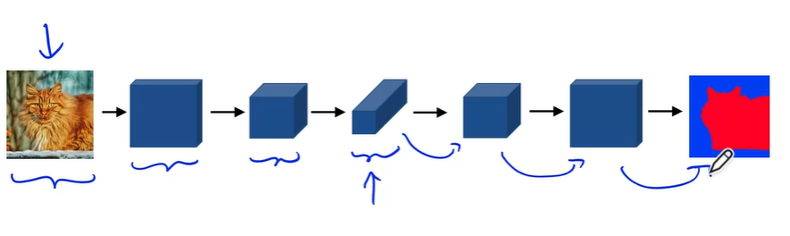
U-Nets can also be thought of as an autoencoder, where the downsampling part, done by the convolutional layers, is an encoder, and the upsampling part, done by transpose convolutional layers, is a decoder. Let’s dive in on how transpose convolutions work to upsample a volume.
Transpose Convolutions
As we mentioned, the key idea behind the transpose convolution is to convolve an input with a filter and generate an output that is bigger than the input.
Let’s say that we have a $2 \times 2$ input, and we’d like to get a $4 \times 4$ output. To get this desired output size, we have to use a $3 \times 3$ filter with padding $p = 1$ and a stride $s = 2$. The basic idea is that we multiply each scalar in the input by the entire filter, element wise, and place the resulting 9 values in the output. As we move the filter in the output, we simply add the values that overlap. There is a great explanation of the transpose convolution here.
U-Net Architecture
The basic idea here is that we use regular convolutions to generate and learn our features, usually reducing the spatial dimensions and adding channels. After this, we blow up the intermediate feature map back into the original dimensions with transpose convolutions. But this is not all.
Another key idea is to use skip-connections, something we have seen before. By using skip connections from the earlier layers, where the spatial information is richer, into the later layers, where the spatial information is poorer but contextual information is richer, we are able to keep the spatial information from degenerating as we go deeper into the network. This key detail is what helps us reconstruct the spatial information into the output, but also use the contextual information used to classify each pixel.
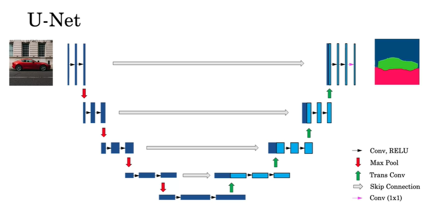
The picture shows why the name U-Net. Notice also that the blocks are the volumes seen from the channel perspective. That is, a wider block has more channels than a thinner block. Let’s start with the first, leftmost, half of the network: the downsampling part:
- We start with our input image of a car.
- We run the input through two convolutional layers, keeping the spatial dimensions the same, i.e. using a “same” padding, but adding some filters. These are the black arrows.
- Then we apply a max pooling operation, and reduce the spatial dimensions by some factor. This is the red downwards arrow.
- We repeat these two operations until we reach the bottom of the picture.
In the bottom of the picture, we have shrunk the spatial dimensions but increased the number of channels by quite a bit, as is usual in CNNs. Our volume has presumably the information needed to classify each pixel, but we have lost the spatial information in the downsampling process. This is where transpose convolutions and skip connections enter the picture.
As we go back up into the right half of the picture, we will do the following:
- Start from our down sampled volume, and apply a transpose convolution to increase the number of spatial dimensions but also reduce the number of filters.
- We concatenate, via the skip connection, the output from the layer before last the max pool operation is applied.
- We apply regular convolutions to this volume, keeping the dimensions the same.
- Repeat this operation until we reach our original spatial dimensions.
In practice, we usually reduce the spatial dimensions by a factor of 2, and then blow them back up by a factor of two every time until we are back to the original spatial dimensions.
Next week’s post is here.