This is the first week of the fourth course of DeepLearning.AI’s Deep Learning Specialization offered on Coursera. This course introduces convolutional neural networks, an extremely popular architecture in the field of computer vision.
This week’s topics are:
- Computer Vision
- Convolution
- Padding
- Strided Convolutions
- Convolutions Over Volume
- One Layer of a CNN
- Simple CNN Example
- Pooling Layers
- Full CNN Example
- Why Convolutions?
Computer Vision
If you can think of any computer vision application today: self-driving cars, medical imaging, face recognition and even visual generative AI; it’s very likely that they’re using some kind of convolutional architecture. Computer vision is a field of computer science that focuses on enabling computers to identify and understand objects and people in images and videos 1. Identification and understanding are nebulous words, but the key thing is that computer vision involves processing digital images and videos. Let’s think about how we could represent an image and use our existing knowledge about neural networks to design a cat classifier.
Say that we want to develop a classifier that processes a digital image, and it outputs the probability that the image is a cat. How are digital images represented usually? A simple, math-friendly, software-friendly way of representing images is as matrices. An image is a grid of pixels, where each pixel has a tuple $(R, G, B)$, where each element represents the color intensity of each channel. If we have a $64\times64$ pixel image of a cat, we would need $64\times64\times3 = 12288$ numerical types to represent the image. But a $64\times64$ pixel image is incredibly tiny. A $1000\times1000$ pixel image, 1 mega-pixel, would require $1000\times1000\times3 = 3,000,000 = 3M$ numerical types to be represented. That’s a lot of numbers, but it gets worse.
If we try to use what we already know, fully-connected feed-forward neural networks, and we set up a single hidden layer with $1,000$ hidden units, then the number of weights will explode. Because we represent each image as a $3M$ vector of features $x_1, x_2, \dots, x_{3M}$, and we are using a fully-connected layer, each feature $x_n$ is connected to each hidden unit. We represent those weights $W^{[l]}$ as a matrix. And that matrix will have dimensions $(1000, 3M)$, which is about 3 billion parameters, and that’s just the first hidden layer.
Sure, we could settle by using smaller images, or compressing larger images - losing detail. But what if there’s a way to avoid the parameter explosion, and, also train a model that overfits less? Remember that big model complexity usually means overfitting. It turns out that convolutions do just that.
Convolution
Convolution in continuous land
When someone mentions convolutions they might be referring to slightly different things. In the field of math called functional analysis, which is the field that uses functions as its units of inquiry, a convolution is an operation between two functions. What is an operation between two functions? Think of differentiation and integration as examples of functional operators.
In this sense, a convolution is a mathematical operation between two functions $f$ and $g$ that produces a third function $f * g$. This third function expresses how the shape of one is modified by the other. It’s defined as an integral:
$$ (f*g) := \int_{-\infty}^{\infty} f(\tau)g(t-\tau)d\tau $$
Perhaps more didactic, there’s a beautiful visual explanation of what a convolution is. It involves plotting $f(t)$ and $g(t - \tau)$ along the $\tau$ axis. As $g(t - \tau)$ is shifted, the convolution $(f*g)(t)$ is plotted, which literally describes the normalized area overlap between the two functions at a particular $t$ value. The integral above is a way to compute that area as the sum of the overlaps over the sliding window.
An animation displaying the process and result of convolving a box signal with itself.

How is this at all related to image processing? Images are not represented as continuous functions, but as discrete objects, i.e., $M \times N \times C$ matrices. It turns out that the discrete equivalent of the integral above is called multidimensional discrete convolution, and this is what people refer to as convolution within the signal-processing and computer vision context.
Convolution in discrete land
So, similar to how we convolve two functions, $f$ and $g$, to find a third function $f * g$, we want to convolve an image and a filter, or kernel. That is, we want to get some output that is, in essence, a filtered image. Why would we want to apply a filter to an image? It turns out that some filters, or kernels, can tell us where the edges are in an image. That seems like a reasonable place to start building a system that can process digital images.
Let’s start by defining a 2D convolution:
$$ g(x,y) = w * f(x,y) = \sum_{dx=-a}^a \sum_{dy=-b}^{b}w(dx,dy)f(x-dx, y-dy) $$
Where $g(x,y)$ is the filtered image, $f(x,y)$ is the original image, and $w$ is the filter kernel. Every element of the filter kernel is considered by $-a \leq dx \leq a$ and $-b \leq dy \leq b$ 2. In essence, this convolves a filter and an image by moving a filter over the image, calculating the sum of all the element-wise products, and setting that as the output for each element in the output matrix. A convolution takes in two matrices and outputs a matrix, but it’s not matrix multiplication. This animation should help clarify what’s going on:

The smaller $3\times3$ matrix is the filter, or kernel, and the large matrix is our image. In this case, instead of having three values representing each pixel, it has one. How to convolve over many channels, or colors in this case, is covered later in the course.
Notice how each of the entries in the output matrix is the result of sliding the filter around the original image, and calculating the sum of all element-wise products. This procedure is what ends up being the discrete equivalent of continuous convolution.
Back to Edge Detection
You might be thinking, how could a matrix (kernel) be used to detect edges? It turns out to be pretty intuitive.
Think about the following $3\times3$ filter:
$$ f = \begin{bmatrix} 1 & 0 & -1 \\ 1 & 0 & -1 \\ 1 & 0 & -1 \end{bmatrix} $$
It turns out that this filter can work as a vertical edge detector. Notice that it’s negatively symmetrical about the middle column. If we convolve this filter by a $3 \times 3$ matrix of equal numbers, the output will be $0$ because the symmetry will cancel everything out. What happens if you convolve this filter with an image that has a vertical edge?
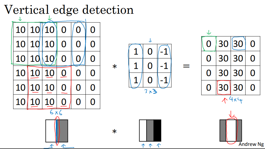
Convolving an image with an edge with this filter will bring up the regions of the original image where there is a gradient of values in the horizontal dimension; thus generating an image that highlights the vertical edges. In this sense, we defined an edge as: a $3\times3$ region in the image where there are bright pixels on the left and dark pixels on the right.
Notice that convolving a $6\times6$ image by a $3\times3$ filter results in a $4\times4$ image. This is the result of convolving without padding, which is covered later.
It might not surprise you that a horizontal edge filter is:
$$ f = \begin{bmatrix} 1 & 1 & 1 \\ 0 & 0 & 0 \\ -1 & -1 & -1 \end{bmatrix} $$
That is, a horizontal edge is a $3\times3$ region in the picture where there are brighter pixels “above” and darker pixels “below”.
But who came up with these numbers? Why not choose $10$ instead of $1$? It turns out that there are a lot of different filters. Think about finding diagonal edges—how would that filter look? But most importantly, how can we know that the filters we use are going to be relevant to our problem domain, i.e., cat classification?
If you think that the convolution explanation is not great, it’s because I don’t really understand convolutions. A great resource is 3Blue1Brown’s beautiful But what is a convolution? video explanation of what a convolution is through the lens of statistics and geometry, and also one that directly explains Convolutions.
Learning the Filters
It turns out that we can unleash all the machine learning knowledge from the previous courses and simply learn the filters that perform best with respect to a cost function. If we define a filter as:
$$ f = \begin{bmatrix} w_1 & w_2 & w_3 \\ w_4 & w_5 & w_6 \\ w_7 & w_8 & w_9 \end{bmatrix} $$
And learn these weights via some optimization algorithm. Do we know which filters will work? No. Can we learn them, whatever they are? Yes!
If we revisit our parameter size estimates, having a $1000\times1000\times3$ matrix representing an image, and a fully connected hidden layer with $1000$ units, then the size of $W^{[l]}$ would be 3 billion. Because in convolution we slide the same filter over the entire image, we just need $10$ parameters (plus the bias) to start building a convolutional layer. We have broken the relationship between our input size and the parameter size of a hidden layer!
The idea of parameter sharing is the powerful idea behind convolutional layers. Not simply because it’s computationally efficient, but also because it helps models generalize better.
Padding
In the example above, we convolved a $6\times6$ image with a $3\times3$ kernel, and got back a $4\times4$ output. This is because once you move the filter to the third column, going left to right, you get to the rightmost border of the image. It turns out that there is a handy formula that we can use to calculate the output dimensions:
$$ \text{output\_dim} = n - f + 1 \times n - f + 1 $$
If we have a $n\times n$ input and convolved it with a $f \times f$ filter, we get out a $n-f+1 \times n-f+1$ output. In the case above: $6 - 3 + 1 = 4$.
But maybe we don’t want to get smaller-sized images after convolving them with our filters. What if we want to convolve them many times? It turns out that there is a solution to this issue, and it’s called padding. Padding will help us deal with the two main downsides of convolving without padding:
- Shrinking output dimensions
- Corner and edge pixels only contribute to very few outputs in the feature map (the output). This means that the pixels around the center of the image will end up being over-represented in the output, relative to the corner and edge pixels.
So what is padding? It’s very simple. Before convolving the image with a filter, you pad the input image, around its edges, with some values. Usually, people use $0$ for the padding, and it’s appropriately named zero-padding. So if we have a $6\times6$ image, and we use a padding of $p=1$, then our padded image will be of dimensions $8 \times 8$. This is because we pad all edges: left, right, top, and bottom. Again, there is a nice formula that allows us to calculate the feature map’s dimensions:
$$ \text{output\_dim} = n+2p-f+1 \times n+2p-f+1 $$
Plugging our example into the formula, we get $6 + 2(1) - 3 + 1 = 6$. Notice that this is the same dimensions as our input. By using padding we were able to keep the convolution output from shrinking. This is called a same convolution, because it preserves the input dimensions. That is, for any given input, you can solve for a padding size that will preserve the dimensions. We can solve for $p$:
$$ \begin{aligned} n+2p-f+1 &= n^* \\ 2p-f+1 &= 0 \\ 2p &= f - 1 \\ p &= \frac{f-1}{2} \end{aligned} $$
So in the previous example, if we have a $3\times3 = f$ filter, then $\frac{3-1}{2} = 1 = p$. This is why a padding of $1$ made our convolution a same one. This is contrasted with valid convolutions, which is where we use no padding.
It turns out that people rarely use even-sized filters, and usually go for odd ones like $3\times3$, $5\times5$, etc.
Strided Convolutions
Another basic building block in CNNs is that of stride. A stride is another tool, like padding, that can be thought of as a hyperparameter of a convolution. A stride is very simple: if we move the filter by $1$ location every time, this is equivalent to using a stride of $1$, $s=1$. We could jump two spaces, or three, or however many we want. However, by using larger strides, we have fewer outputs in the feature map; therefore, it needs to be used with care, otherwise, we get back to our original problem of quickly shrinking the dimensions of our feature maps.
With strides, the handy-formula for the feature map output changes a little:
$$ \text{output\_dim} = \Bigl\lfloor\frac{n+2p-f}{s} + 1 \Bigr\rfloor \times \Bigl\lfloor\frac{n+2p-f}{s} + 1 \Bigr\rfloor $$
Notice that we take the floor, $\lfloor x \rfloor$, to handle the case where the result is not an integer.
So to recap:
- $n \times n$ = image dimensions
- $f \times f$ = filter/kernel dimensions
- $p$ = padding
- $s$ = stride
And the feature map dimensions are given to us by the handy formula:
$$ \text{output\_dim} = \Bigl\lfloor\frac{n+2p-f}{s} + 1 \Bigr\rfloor \times \Bigl\lfloor\frac{n+2p-f}{s} + 1 \Bigr\rfloor $$
Note on difference between convolutions in math vs computer vision. Usually the filter is flipped over the diagonal before convolving. The process of not flipping it is called cross-correlation, while the one where we flip the filter is actually called a discrete convolution. It doesn’t matter whether we flip the filter or not in the context of CNNs.
Convolutions Over Volume
By now, we should have a pretty good grasp on 2D convolution. We have an image, and we convolve it with a filter, and we get some output. We can use padding or a stride different from one, but these are details, and we know how to calculate the dimensions of the output, which is one of the key things to keep in mind; in the same way that it’s very important to keep in mind the dimensions of any neural net. Yet a snag remains: our images are not 2D, but 3D. Our $64\times64\times3$ cat image is a cube. How can we do a convolution over volume?
It turns out that instead of using a square filter, we use a cube filter. That is, if our image is $6\times6\times3$, then we need the number of channels, $3$, to match the number of channels in our filter. Therefore, our filter will have dimensions $3\times3\times3$ if we choose a $3\times3$ filter. Here is an illustration:
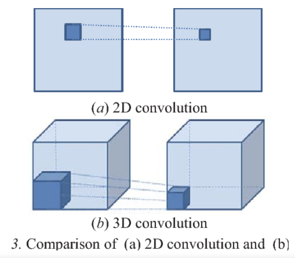
This means that each entry in the output feature map is the element-wise product sum of 27 pairs of numbers; 27 from the image and 27 from the filter, since $3 \times 3 \times 3 = 27$. An important thing to notice is that the number of channels in the output is $1$, and not $3$ as in the input or filter.
But why stop at one filter? We can use as many filters as we want. Think about using one filter for horizontal edge detection, another one for vertical edge detection, and so on. So if we have $n_c^$ filters, we simply stack them together, as long as they are the same dimensions. Let’s say that we have $2$ filters, and they are all dimensions $3\times3\times3$. Then our output will be $n - f + 1 \times n - f + 1 \times n_c^$, where $n_c^*$ is the number of filters used in the layer.
Let’s run by an example using a $6\times6\times3$ input image and two $3\times3\times3$ filters. Convolving a $6\times6\times3$ image with a $3\times3\times3$ filter will result in a $4\times4$ feature map (remember the handy function). Since we have two filters, the feature map will have dimensions $4\times4\times2$. The basic idea being that you can stack multiple feature maps into a cube.
Notice that the (R, G, B) part of the image is usually called channels. It is also called the depth of the image. In the field of machine learning, a multidimensional array might be called a tensor, but this is not really a tensor in the mathematical sense. Just think about channels as the size of the third dimension in the images.
One Layer of a CNN
Getting back to neural nets, we need to fit all these new pieces into the framework we’ve been using throughout the course. We know that ultimately we want to run some optimization algorithm to learn the filter parameters. But before we do that, we need to bring the notation home to make sure that we can apply all the nice tools we developed throughout.
Let’s set up the problem. We have a $6\times6\times3$ image, and that we have two $3\times3\times3$ filters. We convolve each filter with the image, and we get a $4\times4\times2$ output, remember that the $2$ comes from using two filters, so if we had $10$ filters, the output would be $4\times4\times10$. So far so good. The problem is that we don’t have non-linearities! Fear not however, because we can add non-linearities the same way we did before, by using activation functions. The key idea is that we apply an activation function to the output of a convolution between the image and one filter. So after convolving each filter and getting a $4\times4$ output, we pass it through some $a^{[l]}$, our choice of activation function. Not only that, but each filter has its own $b^{[l]}_{n_c^*}$ term, a scalar. So the whole shebang is that we grab each filter, convolve it with the image and get an output. We run that output through an activation function $a^{[l]}$, and then add some $b^{[l]}_{n_c^*}$ bias to the $4\times4$ output, element-wise. Notice that $b^{[l]}_{n_c^*}$ is indexed by the number of filters in the layer $l$, $n_c^*$. This means that if we have a $3\times3\times3$ filter, we don’t have just $27$ parameters, but $28$!
So in this case, the $6\times6\times3$ image plays the role of $a^{[0]}$, our input layer. Remember that we first compute $z^{[1]} = W^{[1]}a^{[0]}+b^{[1]}$. In our case, all the filters we have on our layer play the role of $W^{[1]}$. So the $W^{[1]}a^{[0]}$ term is really the output of a convolution operation. Then we add the biases $b^{[l]}_{n_c^*}$ for each of the filters. Finally, we get $a^{[l]} = g(z^{[1]})$ by passing that output through an activation function (usually a ReLU). This is how we get our final $4\times4$ output. If we have two filters, then the output will be $4\times4\times2$.
This is a good practice question in the course: If we have 10 filters that are $3\times3\times3$ in one layer of a neural network, how many parameters does that layer have? The answer should be even. And again, the truly cool thing about this is that no matter how big the input image is, the number of parameters remains the same. We are no longer in billion-parameter land.
Defining the Notation and Dimensions
If a layer $l$ is a convolutional layer:
- $f^{[l]}$ = filter size.
- $p^{[l]}$ = padding
- $s^{[l]}$ = stride
- $n_c^{[l]}$ = number of filters
Notice that we don’t vary these settings across filters within a layer.
So, layer $l$ will use the output from layer $l-1$; therefore:
- Dimensions of inputs: $n_H^{[l-1]} \times n_W^{[l-1]} \times n_c^{[l-1]}$
- Dimension of outputs: $n_H^{[l]} \times n_W^{[l]} \times n_c^{[l]}$
Where $H$ and $W$ stand for height and width.
Okay, but how do we actually get $n_H^{[l]}$? We use the trusty formula:
$$ n^{[l]}_H = \Bigl\lfloor\frac{n^{[l-1]}_H + 2p^{[l]} - f^{[l]}}{s^{[l]}} + 1\Bigr\rfloor $$
We can do this separately for width and height.
Let’s go over the dimensions of the components of the layer:
- Each filter is $f^{[l]} \times f^{[l]} \times n_c^{[l-1]}$ (notice the channel matching to the previous layer).
- Activations are $a^{[l]} = n_H^{[l]} \times n_W^{[l]} \times n_c^{[l]}$ (the same as the output, of course).
- If we are using mini batch gradient descent, we can describe this with a matrix:
- $A^{[l]} = m \times n_H^{[l]} \times n_W^{[l]} \times n_c^{[l]}$, where $m$ is the mini-batch size.
- If we are using mini batch gradient descent, we can describe this with a matrix:
- Weights are $f^{[l]} \times f^{[l]} \times n_c^{[l-1]} \times n_c^{[l]}$.
- This one is important! $n_c^{[l-1]}$ is the number of channels or filters in the previous layer, while $n_c^{[l]}$ is the number of filters in the current layer.
- The biases $b^{[l]}$ will have one for each filter in layer $l$, therefore it will be of dimensions $1 \times 1 \times 1 \times n_c^{[l]}$, the added dimensions are for broadcasting purposes.
Simple CNN Example
Let’s do a simple example before we go over pooling layers; this should be good practice for calculating the input and output dimensions of the layer.
Let’s start with a $39\times39\times3$ input. We want to convolve it with $10$ filters, where $f^{[1]} = 3, s^{[1]} = 1, p^{[1]} = 0$. Using the trusty formula, we should get an output of dimensions $37\times37\times10$. Remember $\frac{39+2(0)-3}{1} + 1 = 37$, and we have $10$ filters, therefore the output channels are $10$.
Let’s say that we have another convolutional layer $l=2$, and this time we use twenty $5\times5$ filters, so that $f^{[2]} = 5, s^{[2]} = 2, p^{[2]} = 0$. Plugging these numbers into our formula, we start from the last layer’s input size: $37\times37\times10$ and we get this layer’s output dimensions as $17\times17\times20$. Finally, let’s do another layer, $l=3$, with $40$ filters where $f^{[3]} = 5, s^{[3]}=2, p^{[3]} = 0$. Then we end up with an output size of $7\times7\times40$.
Notice how we started with an input of $39\times39\times3$ and end up with a feature map of dimensions $7\times7\times40$; we took a cube and reshaped it into a rectangle. In the case of doing classification, we can run the $7\times7\times40$ output into a $1960$ hidden-unit fully connected layer that runs its output through a softmax or sigmoid.
In summary, the layer types in a CNN are:
- Convolutional Layer |
CONV - Pooling Layer |
POOL - Fully connected Layer |
FC
Pooling layers are discussed next and remain a key part of CNNs.
Pooling Layers
Pooling layers reduce some layer’s output dimension by applying an aggregating procedure, usually taking the max or average over some region in the output. This is good for two main reasons: smaller outputs are more computationally efficient. However, unlike the output shrinking from filters, the aggregating procedures can boost certain features down the network.
A pooling layer works similar to a convolutional layer. An example of $2\times2$ max pooling is shown here:

Each of the outputs in the feature map is simply the maximum value in the input’s region overlaid by the filter. We can still use our trusty formula to calculate the output sizes.
A key thing to notice is that pooling layers have no parameters. That is, they only have hyperparameters, $f$ and $s$—that is, their size and the stride. Additionally, another hyperparameter is whether the layer is a max-pooling layer or average-pooling layer. Max-pooling is a lot more popular in the CNN literature.
Full CNN Example
This example goes over a CNN architecture similar to that of LeNet-5, a legendary architecture proposed by Yan LeCun in 1998. The network was implemented to do character recognition originally.
The architecture is as follows:
- Input: $32\times32\times3$
CONV 1: $f=5, s=1$. Outputs: $28\times28\times6$MAXPOOL 1: $f=2, s=2$. Outputs: $14\times14\times6$CONV 2: $f=5, s=1$. Outputs: $10\times10\times16$MAXPOOL 2: $f=2, s=2$. Outputs: $5\times5\times16$FC3: $120$ units. The weights $W^{[FC3]}$ has dimensions $(120, 400)$. Where $400 = 5\times5\times16$.FC4: $84$ units. The weights $W^{[FC4]}$ has dimensions $(120, 84)$Softmax: The final output layer with $C=9$ classes, one for each digit.
A couple of details:
- In the literature, a convolutional layer is usually referred to as a
CONVlayer followed by aPOOLlayer. SoCONV 1andMAXPOOL 1can be referred to as a single layer. - The dimensions of the feature maps tend to decrease. That is, $n_H, n_W$ go down as we go deeper in the network.
- The number of channels tends to increase; that is, $n_C$ goes up as we go deeper in the network.
Here is a table with the dimensions for each layer and also the number of parameters. Verifying the number is a great exercise to test our understanding:
| Activation shape | Activation size | # Parameters | |
|---|---|---|---|
| Input | (32, 32, 3) | 3,072 | 0 |
| CONV1 $(f=5, s=1)$ | (28, 28, 6) | 4,704 | 456 |
| POOL1 $(f=2, s=2)$ | (14, 14, 6) | 1,176 | 0 |
| CONV2 $(f=5, s=1)$ | (10, 10, 16) | 1,600 | 2416 |
| POOL2 $(f=2, s=2)$ | (5, 5, 16) | 400 | 0 |
| FC3 | (120, 1) | 120 | 48,120 |
| FC4 | (84, 1) | 84 | 10,164 |
| Softmax | (10, 1) | 10 | 850 |
Notice how the activation sizes decrease through the layers. Also, notice how around 94% of all the parameters in the network are part of the fully connected layers. This network has a grand total of $62,006$ parameters, which is a lot less than hundreds of millions.
Why Convolutions?
Unfortunately, there is no single reason as to why convolutions work so well. However, there are two probable reasons:
- Parameter sharing: Since you use the same filter to convolve it across different parts of the image, you can use the same filter many times. This is related to translational invariance, the idea that a CNN is robust to shifted or distorted images.
- Sparsity of connections: Each output value depends only on a few inputs. This is a mark of low complexity, and it might have an effect similar to regularization; therefore, helping avoid overfitting.
Next week’s post is here.